What Color is it?
What Color is it?
ANDREW T. YOUNG
1 Abstract
Color vision provides low-resolution spectrophotometric
information about candidate materials for planetary
surfaces that is comparable in precision to wideband
photoelectric photometry, and considerably superior to
Voyager TV data. This paper briefly explains the basic
concepts, terminology, and notation of color science. It
also shows how to convert a reflectance spectrum into a
color specification. An Appendix lists a simple computer
subroutine to convert spectral reflectance into CIE
coordinates, and the text explains how to convert these
to a surface color in a standard color atlas. Target and
printed Solar System colors from a recent article (Young,
1985) are compared to show how accurate the printed colors
were.
2 INTRODUCTION
Color vision powerfully molds our ideas about planetary
surface materials. Although the color of a substance
provides only partial information about its spectrum, its
spectrum cannot match a planet's if their colors differ.
Hence, to be able to think of appropriate candidate
materials, you must first see the correct planetary colors.
If the stuff you have in mind doesn't have the right color,
you don't have the right stuff.
This problem has been vividly illustrated recently
by the false colors on published Voyager pictures that
misled people into looking for red and orange candidate
materials for the surface of Io, which is actually greenish
yellow. Io was described as red or orange not only by the
popular press, but by prominent scientists and respected
science writers. For example, Henbest and Marten (1983)
call Io “orange”, and refer to a false-color picture as “true
color”. The book produced “in association with the Royal
Astronomical Society” by Hunt and Moore (1981) says of Io,
“The color was red and orange.” (As one of these authors was
a member of the Voyager TV team, this statement refutes the
claim that team members, at least, did not believe those
colors.) Morrison et al. (1982) refer to “Io's … orange
surface” in their famous book, “Powers of Ten.”
In this paper, I hope to provide planetary scientists
with enough guidance to the literature of color science
to prevent such mistakes in the future. The amount of effort
required to find colors from spectra is really quite small;
I was able to determine the first correct color on Io in
less than a week after deciding to do so, and most of this
time was spent searching an unfamiliar literature for the
information I needed. If a reflectance spectrum is already
available in tabular form, the corresponding surface color
can be found in about an hour with a pocket calculator.
3 VADE MECUM
Although color science has existed in roughly its present
form for over a century, most scientists know much less
about color than they think they do. For example, a recent
book (Malin and Murdin, 1984) on the “Colours of the Stars”
not only presents false-colored pictures as true ones, but
even gives a completely muddled “explanation” of color
itself. Such widespread ignorance may explain why no
correctly colored picture has ever been published from
spacecraft television data, although some recent
approximations (Young, 1985) are fairly close.
Part of the difficulty is due to a common experience in
the educations of physical scientists: looking into a
spectrometer, and seeing that monochromatic lights of
different wavelengths have different colors. Many people
incorrectly suppose that there is a one-to-one relation
between wavelength and color, or that such a relation
exists between spectral energy distribution and color.
But even the existence of a unique color (under fixed viewing
conditions) for each monochromatic wavelength or each
spectral distribution does not imply that a converse
relation exists. In fact, it cannot, because color spaces
have lower dimensionality than the vector spaces needed
to represent spectra; infinitely many spectra necessarily
map into the same color.
For example, the fact that only the longest visible
wavelengths in the spectrum appear reddish may lead to a
false assumption that “red” implies “only long wavelengths”;
actually, all spectral reds are slightly orange, and the
“unique” or “invariable” red that looks neither bluish nor
yellowish is a non-spectral color, complementary to the
cyan elicited by wavelengths near 494 nm (Kelly, 1943; Le
Grand, 1957, pp. 211-212; Committee on Colorimetry, 1963,
p.106; Wyszecki and Stiles, 1982, pp. 424, 456). “Pure red”
contains some short-wavelength light.
Another difficulty is the physical scientist's habit of
externalizing reality. Thus, many of us wrongly assume
that color is a property of electromagnetic radiation,
rather than of the human visual system. But color really
lies within the observer, and not “out there” in the light.
Even Newton (1730; pp. 123-125) realized that “if at any time
I speak of Light and Rays as coloured or endued with Colours,
I would be understood to speak not philosophically and
properly, but grossly, and according to such Conceptions
as vulgar People … would be apt to frame. For the Rays to
speak properly are not coloured. In them there is nothing
else than a certain Power and Disposition to stir up a
Sensation of this or that Colour.”
The study of this sensation of color now belongs to
the broader science of vision, an interdisciplinary area
involving psychophysics, physiology, biochemistry,
neuroanatomy, and other fields of medical and biological
science, in addition to our more familiar areas of physical
optics, radiometry, photochemistry, and optical
instrumentation. These disparate disciplines are so
intimately mixed in color science that one cannot easily
predict where to find a particular book; for example, Le
Grand's (1957) text is filed in our library with books on
physiology and biochemistry, although the author's preface
states that “the point of view is essentially that of the
physicist”!
Similarly, although Boynton (1979) states that
his book emphasizes physiology, it is classified under BF
(Psychology) by the Library of Congress.
The psychological aspect of color science does not mean
that it is all “subjective” (in the sense of “personal” or
“unreliable”), for as Boynton (1979; p.333) points out,
“data of astonishing reliability” can be generated under
controlled conditions.
[Indeed, Appendix A shows that the
precision of visual colorimetry is at least as good as
that of the (B-V) photoelectric color index, for planetary
colors.] It does, however, mean that one must distinguish
clearly between the light stimulus and the color response
it elicits.
Under fixed conditions, a particular spectral
distribution does elicit a unique color sensation. Thus
it is possible to determine the apparent color of a surface
from its spectral reflectance. As the spectral reflectances
of planetary surfaces are fairly well determined, their
colors can be determined also. A standard procedure for
doing this was developed in the 1940's, and will be briefly
described here.
This standard procedure was followed and very briefly
described by Huck et al. (1977), who correctly determined
colors on Mars. Unfortunately, they then failed to
reproduce
the correct colors in the accompanying color plates.
Furthermore, the completely false and misleading colors
on all pictures published by the Voyager TV team (Smith et
al., 1979a,b) — including a picture labelled “nearly
natural color” (Smith et al., 1979b, p.938) — indicates
that the cursory explanation given by Huck et al. (1977) was
inadequate to educate the planetary community.
Hence, to make the explanation comprehensible, I have
prefaced it by a short tutorial on color science. Kuehni's
(1983) book is a more detailed, but quite short and readable
introduction. Many basic concepts are briefly described
and well illustrated in color in Kelly and Judd (1976), and
in the excellent Kodak Publication E-74, “Color as Seen and
Photographed” (now, unfortunately, out of print). Readers
who want to learn more about color should then consult a
standard text or reference such as the books by Le Grand
(1957) or MacAdam (1981), or that published by the Committee
on Colorimetry (1963). Those who are uncomfortable with the
vector-space description used here will be happier with
Boynton's (1979) introduction, though it barely mentions
colorimetry. The current status of the science is fully
reviewed by Wyszecki and Stiles (1982); this huge book
contains nearly 1300 references.
4 COLOR PERCEPTION
4.1 Color and Appearance
To begin with, we must distinguish color from other
aspects of appearance, such as gloss, texture, and luster.
Failure to do this led Malin and Murdin (1984; pp. 35, 137)
to call “gold” a color; the metal has a yellow color, but
(unlike most ordinary surfaces) a metallic luster. The
Committee on Colorimetry (1963, p.58) calls such use of the
names of materials for color names “confusing”, pointing
out that “metallic luster is a characteristic of objects
distinguishable from color,” and recommends that “names
suggesting such characteristics should not be used as
color names.”
4.2 Modes of Color Perception
We must also recognize the difference in appearance
between surface colors, volume colors (as in colored filter
glasses), and colored lights. These and other “modes of
appearance” are compared by the Committee on Colorimetry
(1963, p.151). Here, we are mainly interested in the colors
of surfaces (in particular, planetary surfaces).
4.3 Related and Unrelated Colors
The perceived color elicited by a fixed stimulus depends
not only on the state of adaptation of the eye, but also on
the visual context in which the stimulus appears. The
colors of lights seen in isolation against a black surround
are seen in the “aperture” or “film” mode. These are “unrelated
colors”; this is how we usually see planetary colors against
the dark sky in a telescope eyepiece. Colors seen this way
appear to have no black content. Without a white reference
to show the intensity of the incident illumination, they
appear as brighter or dimmer lights on a open-ended scale
without white or black limits. Thus, the Moon appears “bright”
and may seem “white” in the telescope, though it is as dark
as the average asphalt paving surface. Similarly, Mars
looks yellow-orange in the telescope, though it is really
yellowish brown.
In a normal environment that contains familiar objects
and other visual cues, such as specular reflections of the
light source (D'Zmura and Lennie, 1986; Lee, 1986) the eye
and brain adapt to and compensate for the color of the
illumination. Colors seen in this mode are called “related
colors”. Here a definite brightness level appears “white”;
brighter surfaces appear self-luminous or fluorescent.
Instead of the “brightness” scale of lights, we perceive
“lightness” of surfaces relative to the white standard.
4.4 Color Constancy
Under such conditions, we experience “color constancy”
for a given object, even though the spectral radiance it
sends to the eye depends strongly on the quality and
brightness of the illumination (see D'Zmura and Lennie,
1986; Maloney, 1986; Lee, 1986; and other papers in the same
issue of J.O.S.A.) Thus, a wide range of different illuminants
can elicit nearly the same (related) color perception from
an object, although the stimuli it presents to the eye may
be very different.
On the other hand, the same spectral distribution
entering the eye can be perceived as very different colors
in different contexts. For example, you might perceive the
light of a candle flame scattered by this page as “white”,
if you were adapted to that light; as “orange”, if you had
just come from a room lit by fluorescent lamps; or as “brown”
or “black” if you were standing in daylight, and saw the
dimly-lit page through a small hole in a window shade.
Although these contextual and adaptive effects mean
there is generally no fixed relation between spectral
distribution and perceived color, a surface of given
spectral reflectance
does
have a fixed, determinable color
under
fixed
viewing conditions. Critical color comparisons
require both a fixed angular size of stimulus and a fixed
surround (usually a neutral gray of about the same lightness
as the samples to be compared), as well as a fixed spectral
illuminant.
In particular, a surface of given spectral reflectance
has a fixed and reproducible (i.e., “constant”) related color
when viewed in typical daylight conditions. The method
for determining that color from the surface's spectral
reflectance is described below. But first, we must consider
color nomenclature.
4.5 Color Spaces
All visible colors can be arranged in a continuous three-
dimensional sequence or “color space”. This empirical fact
has been known for centuries. However, the choice of
coordinate axes is quite arbitrary, and a wide variety of
systems has been used (cf. Wyszecki and Stiles, 1982,
pp. 164-169, 486-513, and 824-884). Some of these are
illustrated by Kelly and Judd (1976).
Human color space is three-dimensional because our eyes
contain three types of cone-shaped receptors, each with
its own type of spectral response, that contribute to color
vision. We may crudely describe the sensations they produce
as “blue”, “green”, and “red”. However, the detected signals
are immediately processed in the eye and brain to yield a
brightness channel (roughly, the sum of the green and red
cone signals); a red-green channel (their ratio); and a
blue-yellow (blue vs. red + green) channel. These “opponent
mechanisms” modify the signals before we perceive them,
so perhaps the most natural dimensions of color space are
black/white, red/green, and yellow/blue. Such natural basis
vectors appear in both psychophysical (Krauskopf et al.,
1982) and physiological (Derrington et al., 1984) experiments.
The black/white mechanism helps explain why unrelated
planetary colors seen in the telescope show no black
content: adaptation to the black surround drives this
channel toward white. On the other hand, when we see typical
planetary materials as related surface colors in the
laboratory, those with reduced lightness can “cause new
sensations to appear, especially in the region of orange,
yellow, and greenish yellow. If the lightness of the
specimens is low these colours appear as chestnut, brown
and olive-green respectively” (Le Grand, 1957, p.220).
Similarly, Kelly and Judd (1976) say that “… the term
yellow is commonly used to designate not only a certain
hue range but also a high lightness range within this hue
range. Dark colors of the same hue as yellow are commonly
termed olive or olive brown. Common usage limits the term
orange even more strictly; it is taken to refer not simply
to a range of yellow-red hues but also to a medium-lightness
range and a high saturation range. Colors of the same hue
but of lower lightness and saturation than the orange
range are called browns.”
Because so many planetary surfaces are brown, it is
necessary to emphasize that this color is perceived when
any dark yellowish surface is seen as a related surface
color. It is not, as Malin and Murdin (1984; p.137) say, a
“non-spectral” color; that term is reserved for the purple
hues that cannot be matched by any mixture of monochromatic
and white light. (They compound the confusion by saying
that “non-spectral … means that it cannot be made simply
by combining red, green, and blue lights in an additive
process.” The non-spectral purples are in fact made by
adding red and blue lights; moreover, as will be shown below,
there are even spectral colors that cannot be matched by
adding red, green, and blue lights! They have confused the
distinction between surface and aperture modes with the
difference between spectral and non-spectral colors.)
4.7 Munsell Renotation for Surface Colors
The system of arranging surface colors that is best
known in the United States is that introduced by A.H.Munsell
about 1905; with minor modifications, the same system is
available today from Munsell Color (Macbeth Division of the
Kollmorgen Corp., 2441 N.Calvert St., Baltimore, MD 21218).
The standard colors in this system are available as both
glossy and matte-finish painted papers; various sets of
these colors are published in different editions of the
Munsell Book of Color.
The Munsell system arranges all colors cylindrically
about a vertical axis whose direction represents the
sensation of lightness. A pure white magnesium oxide block
is assigned Munsell value 10/; value 5/ represents a medium
gray; and value 0/ is perfectly black. The physical quantity
that is related to Munsell value is visual reflectance.
However, the nonlinearity of the human visual system makes
the Munsell value scale lie between the square and cube
roots of reflectance, so that value 5/ corresponds to about
20% reflectance. The precision of visual judgments is one
or two tenths of a Munsell value step (Nickerson, 1947,
p.167; Kelly and Judd, 1976, p.A-13). This corresponds to
about 4% precision in visual reflectance, for typical
surfaces.
All shades of gray form the central vertical axis of the
cylindrical Munsell coordinate system. The azimuthal
coordinate is hue (red, yellow, green, blue, purple, etc.),
which is what is often meant by the word “color” in casual
conversation. The five main hues just named are equally
spaced; between them lie secondary combinations such as
YR for “yellow-red” and GY for “green-yellow”. Each of the
10 named hues is subdivided into 10 numerical subclasses,
rather like stellar spectral types (which are also based
on visual estimates). Thus, a pure red has hue 5R; orange
is 5YR; and the borderline between them is 10R or 0YR. The
precision of hue matches for experienced observers is
about 1/4 Munsell hue unit for highly saturated colors
(Kelly and Judd, 1976); a more typical value is 0.6 in hue
(Nickerson, 1947).
The amount by which a color differs from gray (i.e., the
radial coordinate in the Munsell system) is called “chroma”.
A more familiar word for a closely related concept is
“saturation”. The pure spectral colors have maximum chroma,
which is about 20 (because the most saturated red pigment
available to Munsell had about half this saturation and
was given chroma 10; see p.74 of Birren, 1969). White,
grays, and black have chroma zero, and are thus sometimes
called “achromatic colors”, to distinguish them from the
“chromatic colors”. The precision of visual color matching
between observers is about 0.3 Munsell chroma unit.
The complete Munsell specification for a surface color
is given as Hue Value/Chroma. For example, 5Y 8.5/12 is a
medium yellow hue (5Y) of high lightness (value 8.5) and
saturation (chroma 12), about the color of dandelion blooms.
The conventional representation of the Munsell system is
left-handed; i.e., if the value axis increases upward, the
hue subdivisions increase numerically clockwise, looking
down along this axis. Hue-chroma planes (i.e., surfaces of
constant value) are drawn with the 5R ray toward the top of
the page, with yellow, green, blue, and purple following in
clockwise order.
Munsell notations are widely used in industry, not only
because they are easily determined by quick visual
comparisons with Munsell color standards, but also because
they provide quantitative information of high precision.
Appendix A
shows that the precision of visual color matching
is comparable to or better than that of wideband
photoelectric systems such as UBV, and much better than
spacecraft television systems have done. The utility of
visual color measurement has been recognized in some
fields, such as geology, but is largely neglected by
planetary scientists.
Munsell renotations are nearly uniformly spaced
perceptually. The original notations were established
visually, without any reference to spectrophotometry.
However, spectrophotometric data were used 40 years ago to
make the system smoother in a stimulus color space,
described below. This minor revision caused the
“renotations” to differ very slightly from the original
notations in older editions.
The December, 1940, issue of J.O.S.A. was devoted
to a detailed investigation of the old Munsell system,
including the history of its development. The Munsell
renotations were adopted by the American Standards
Association in 1951 (ASA-Z58.7.1,2,3). The system is
described and well illustrated in “Webster's Third New
International Dictionary of the English Language
Unabridged”, under the entry “color”. Birren (1969) gives a
thorough description of Munsell's system.
5 STIMULI AND COLORIMETRY
5.1 Illumination and Surface Colors
The spectral energy distribution of the light stimulus
reflected from a surface to the eye depends both on the
spectral reflectance of the surface and on the spectral
energy distribution of the light that illuminates the
surface. The Commission Internationale de l'Eclairage (CIE)
established three standard illuminants for colorimetry
in 1931. Illuminant A represents light from the full
radiator (black body) at 2856 K, and is closely approximated
by a tungsten-filament lamp with this correlated color
temperature; Illuminant B was intended to represent direct
sunlight, excluding the light of the blue sky; and Illuminant
C was intended to represent average daylight (a mixture of
transmitted sunlight and diffuse skylight).
Subsequently, Illuminant C was found to be slightly
deficient for some purposes, mainly connected with
fluorescent materials. Planetary surfaces are not
appreciably fluorescent, so this problem is minor; and in
any case we will need to use a great deal of work done with
Illuminant C. However, it will eventually be replaced by
the better daylight approximation designated as D65.
5.2 Stimulus space and metamerism
Just as we have used the Munsell notation to describe
perceived surface colors, we may define a three-dimensional
color space for the spectral radiance functions of the
colored stimuli. (For any definite illuminant, such as CIE
Illuminant C, this is equivalent to using the spectral
reflectance functions for surface colors.) However, even
if we restrict attention to bounded, continuous functions,
this set is infinite in dimension (Hilbert space; see
Parkkinen and Jaaskelainen, 1987). Distinguishable color
stimuli are only the projection of this infinite-
dimensional space of spectra onto a three-dimensional
subspace of colors. In this respect, color vision is like
3-color broadband astronomical photometry (Young, 1974a).
The projection vector (whose components are continuous
functions of wavelength, and which is orthogonal to the
three-dimensional subspace of color vision) can be
determined only by measurements made by human observers,
to determine sets of physically different color stimuli
that are visually identical. Such stimuli are called
metameric, or are said to be metamers of one another. Any
stimulus that is not monochromatic has an infinite number
of metamers.
The spectra of metamers differ by functions whose
projection into human color space is null. Table I(3.8.2)
of Wyszecki and Stiles (1982) gives 27 such “metameric
blacks”, and their Fig. 7(3.8.2) shows 12 wildly different
spectral reflectance functions of surfaces that would
appear the same shade of gray under illuminant C.
Fortunately, statistical studies of many natural and
artificial surfaces (e.g., Maloney, 1986; Parkkinen and
Jaaskelainen, 1987) show that well over 90% of the variance
among real reflection spectra is accounted for by the
first 3 principal components. Thus, even though about seven
parameters are needed to produce an essentially perfect
fit to such data, so that about seven dimensions are in
fact required to represent actual surface spectral
reflectance functions accurately, it turns out that the
three dimensional subspace of color vision captures the
bulk of significant information about real colored surfaces.
As Maloney (1986) points out, the spectral reflectances
of real surfaces are band-limited functions, due mainly
to the width of electronic absorptions in solids. That is
why only about seven dimensions are needed to represent
the spectral reflectances of real surfaces. This
band-limited character has allowed the broadband filters
used in spacecraft TV systems to capture most of the
significant information about planetary surface spectra.
It also explains the utility of broadband photometry in
characterizing asteroid surfaces. Thus, the undersampling
of object spectra by all these systems, including the eye,
does not produce severe aliasing problems; metamerism is
not a serious nuisance in practice.
5.3 Color matching and primaries
The metamers can be found by means of color-matching
experiments. In a typical experiment, three highly saturated
lights of widely different hues are chosen as “primaries”.
The choice of primaries is quite arbitrary; often
monochromatic or nearly monochromatic lights are used.
It turns out that any color can be matched by some linear
combination of these primaries.
However, it is
not
true, as Malin and Murdin (1984; pp. 35,
60-61) assert, that “All the colours of the spectrum …
can be mimicked by combinations of different intensities
of … blue, green, and red,” nor that “coloured lights can
be mixed to give pure spectral hues”. The “linear
combinations” in these cases involve negative coefficients;
spectrum colors other than those in the set of primaries
would require negative amounts of some complementary
primary, to be matched by direct addition. As negative
intensities do not exist, this is impossible.
However, the negative coefficients can be evaluated by
modifying the matching experiment. If the appropriately
scaled amounts of the primaries are denoted by A, B, and C,
and some test stimulus D is equivalent to A + B − C, we note
that D = A + B − C can be rearranged to read C + D = A + B.
Hence, the additive mixture of lights A + B should match the
additive combination C + D. Thus, if we add the primary
requiring a negative coefficient to the test stimulus, we
can extend the experiment to include colors outside the
region of direct additive combinations. (If the primaries
are not monochromatic, two of them may need such treatment
to match certain monochromatic stimuli.)
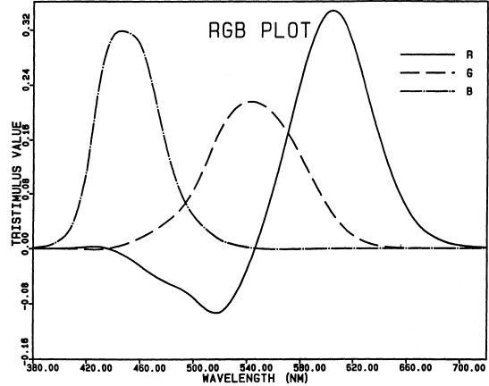
5.4 Tristimulus values
 The amounts of the three primaries required to match a
given color are called its “tristimulus values”. Negative
tristimulus values occur in all color-matching experiments
with physically realizable primaries (MacAdam, 1981, p.11;
see Fig. 1). The reason for this is well explained by
Boynton (1979, pp. 128-144); briefly, it is due to the
overlap of the cones' spectral responses, which makes most
monochromatic stimuli excite more than one kind of receptor.
There is no light, for example, that stimulates only the
“green” cones and no others.
The amounts of the three primaries required to match a
given color are called its “tristimulus values”. Negative
tristimulus values occur in all color-matching experiments
with physically realizable primaries (MacAdam, 1981, p.11;
see Fig. 1). The reason for this is well explained by
Boynton (1979, pp. 128-144); briefly, it is due to the
overlap of the cones' spectral responses, which makes most
monochromatic stimuli excite more than one kind of receptor.
There is no light, for example, that stimulates only the
“green” cones and no others.
Fig. 1.
Spectral tristimulus values of monochromatic lights
of equal power, with respect to monochromatic primaries
at 700 nm (approximately a red-filtered tungsten lamp),
546.1 nm (the mercury green line), and 435.8 nm (the mercury
blue line), for the CIE 1931 standard observer [see Table
I(3.3.3) of Wyszecki and Stiles, 1982]. At each wavelength,
the ordinates show the amounts of the three primaries
required by the standard observer to match a light of that
wavelength and fixed power in a two-degree field. Note that
these color-matching functions for real primaries have
negative lobes, as discussed in the text. Notice also that,
at each primary wavelength, the curves for the other two
primaries cross at zero. For example, at 546.1 nm, the
green line alone matches itself, so the required amounts
of the red and blue primaries are zero.
Any color stimulus can be represented by a point in a
three-dimensional “tristimulus space” whose coordinates
are its three tristimulus values. If actual lights are
used as primaries, all color stimuli project into points
that are contained in a half-space (i.e., they lie on one
side of a plane through the origin, which is the zero
stimulus.)
Because the cones' spectral response functions overlap,
the subspace of real colors does not fill this half-space,
but define a cone whose vertex is the origin and whose base
is a convex curve. Spectrally pure lights lie along the
elements of this cone. The colors that can be produced by
additively combining any three primary lights fill a
triangular pyramid lying entirely within the cone; each
primary lies along one edge of the pyramid [see Fig.
1(3.2.2), p.121 of Wyszecki and Stiles (1982)]. No matter
what three lights are used as primaries, there are always
colors lying between the pyramid and the (convex) cone that
cannot be produced with positive tristimulus values. These
are the colors that require negative values of one (or two,
if the primaries are not spectrally pure) of the primaries.
5.5 Color-matching functions
If we plot the tristimulus values required to match
monochromatic lights of constant power as functions of
wavelength, we call the resulting functions the “color-
matching functions” with respect to the chosen primaries.
Thus,
Fig. 1 shows the color-matching functions with respect
to primaries at 700 nm, 546.1 nm, and 435.8 nm. Color-
matching functions are conventionally denoted by lower-
case letters, with an overbar as a reminder that they refer
to the same power at each wavelength. Thus, the CIE
color-matching functions with respect to the primaries R,
G, and B shown in Fig. 1 are denoted by
r̅,
g̅, and
b̅.
The choice of primaries is quite arbitrary, so long as
their vectors in color space are not coplanar. Each set of
primaries is a different set of basis vectors for the same
three-dimensional color space. Any three linearly
independent combinations of these color-matching functions
span the same three-dimensional subspace of all possible
spectral functions, and hence are also color-matching
functions (with respect to a new set of primaries).
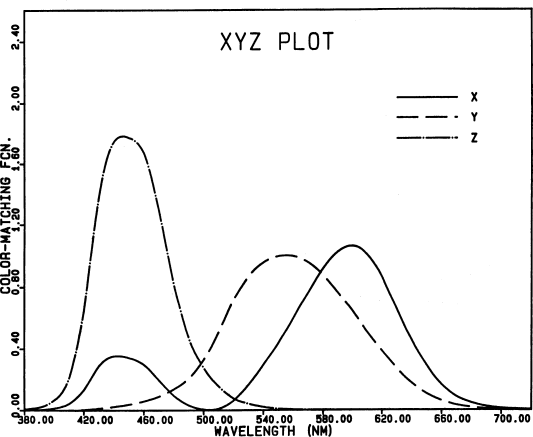 In particular, we can choose combinations of color-
matching functions that are entirely positive. These are
much more convenient to work with (for example, they can
serve as spectral response functions in a colorimeter),
but they refer to primaries that lie outside the range of
physically realizable colors. In 1931, the CIE adopted such
a set of positive color-matching functions, denoted by
x̅,
y̅, and
z̅ (see Fig. 2), which have been so useful and accurate
a representation of normal human color vision that they
remain in standard use today.
In particular, we can choose combinations of color-
matching functions that are entirely positive. These are
much more convenient to work with (for example, they can
serve as spectral response functions in a colorimeter),
but they refer to primaries that lie outside the range of
physically realizable colors. In 1931, the CIE adopted such
a set of positive color-matching functions, denoted by
x̅,
y̅, and
z̅ (see Fig. 2), which have been so useful and accurate
a representation of normal human color vision that they
remain in standard use today.
Fig. 2.
The 1931 CIE color-matching functions, which refer
to non-physical primaries called X, Y, and Z. Their relation
to the R, G, B primaries is discussed in Section 3.3.3 of
Wyszecki and Stiles (1982). Fig. 4(3.3.3) in their book
shows the X, Y, Z tristimulus space; the cone containing all
real colors lies entirely within the first octant of (X, Y,
Z) space. Notice that all spectral colors (and hence, all
real colors) have only positive tristimulus values with
respect to these non-physical primaries.
The CIE primary X represents a red stimulus more saturated
than any real stimulus, and of hue complementary to 496 nm;
Y is a green primary the same hue as monochromatic light
at 520 nm, but more saturated; and Z is a blue primary more
saturated than 477-nm light (MacAdam, 1981, p.11). The
color-matching function y̅
was chosen to be the so-called
“visibility” or “luminosity” function of the eye, which
shows the relative ability of each wavelength to produce
the sensation of brightness. The CIE color-matching functions
are tabulated in all reference works on colorimetry (e.g.,
Le Grand, 1957, p. 454; MacAdam, 1981, pp. 13, 59; Wyszecki
and Stiles, 1982, pp. 725-753).
Because the color-matching functions show the relative
amounts of the primaries required to match monochromatic
light at each wavelength, the tristimulus values (X, Y, Z) of
any spectral distribution r(λ)
are just the wavelength
integrals of the products of r(λ)
with each of the
color-matching functions
x̅,
y̅, and
z̅,
respectively. In
practice, these integrals are well approximated by sums
(see Chapter 5 of MacAdam, 1981).
Appendix B gives a simple
FORTRAN 77 subroutine for computing CIE tristimulus values of
surfaces under Illuminant C from spectral reflectances.
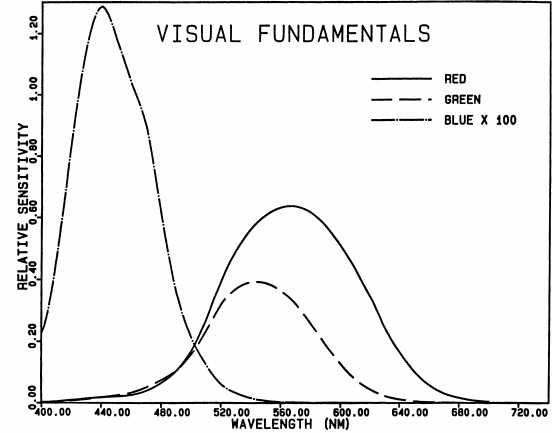 Notice that these color-matching functions need not
resemble the fundamental response functions of the
receptors in the eye, but are just some linear combinations
of them. Indeed, color-matching data from normal individuals
do not suffice to determine the eye's primary response
functions. However, data from color-deficient individuals
can be used to deduce the action spectra of the missing
visual pigments, and these functions agree reasonably
well with absorption spectra measured
microspectrophotometrically on individual cones (see Fig. 3).
Notice that these color-matching functions need not
resemble the fundamental response functions of the
receptors in the eye, but are just some linear combinations
of them. Indeed, color-matching data from normal individuals
do not suffice to determine the eye's primary response
functions. However, data from color-deficient individuals
can be used to deduce the action spectra of the missing
visual pigments, and these functions agree reasonably
well with absorption spectra measured
microspectrophotometrically on individual cones (see Fig. 3).
Fig. 3.
Visual fundamentals, according to Smith and Pokorny
(1975). The blue fundamental has been multiplied by a
factor of 100, because the absolute blue sensitivity of the
eye is very low.
5.6 Chromaticity Coordinates and Dominant Wavelengths
Lights of the same spectral distribution but different
brightness have tristimulus values that differ only by a
constant factor. It is conventional, for convenience in
two-dimensional plotting, to normalize the X and Y
coordinates by the sum (X + Y + Z); the normalized coordinates
and
are called “chromaticity coordinates”. Two lights of the
same color except for brightness have the same chromaticity
coordinates. In dealing with colored lights, it is often
acceptable to ignore that third dimension of color space,
so a two-dimensional chromaticity diagram shows the
information of interest.
Similarly, we can compute the chromaticity coordinates
of surfaces from the spectra of the light they reflect, if
the spectral distribution of the illuminant is given. Two
surfaces that differ only in lightness under a given
illuminant have the same chromaticity coordinates. In
this case, using a two-dimensional chromaticity diagram
may reject important information; for example, “pieces of
chocolate and orange peel have the same chromaticity
coefficients and differ only in lightness” (Le Grand, 1957,
p.220). Also, notice that because the spectral distribution
of the illuminant is multiplied by the spectral reflectance
of the surface within the integrand, two surfaces that are
metamers under one illuminant are generally not metamers
under other illuminants.
The chromaticity coordinates of CIE Illuminant C are
(x = 0.3101, y = 0.3163). Any point along a line joining
this “white” stimulus to a point on the spectrum locus
represents a color that can be matched by a mixture of
white light from Illuminant C and monochromatic light,
whose wavelength is called the “dominant wavelength” of
the colors along the radial line. The fraction of
monochromatic light in this mixture is called the
“excitation purity”; it is the fraction of the distance
from C to the spectrum locus where the point falls on the line.
Thus, the CIE chromaticity space has orthogonal Cartesian
coordinates (x, y, Y), and is usually drawn with the Y axis
vertical. The axes form a right-handed set, so that the
spectral hues follow a counterclockwise order from red
to blue in an (x, y) plane. Notice that this is the reverse
of the usual Munsell ordering.
6 FROM CHROMATICITY TO COLORS
It is essential to realize that chromaticity coordinates
alone specify nothing beyond metamerism. That is, two
surfaces with the same (x, y, Y) coordinates in a given
illuminant, or two lights with the same values of (X, Y, Z),
appear identical to the CIE standard observer. The
coordinates themselves do not tell us
what
colors the eye
sees; nor are equally spaced colors in chromaticity space
at all equally spaced perceptually.
However, the mapping of points from a stimulus space
(e.g., CIE chromaticity coordinates) to a perceived color
space (e.g., Munsell renotation) for given viewing conditions
can be determined empirically. Fortunately, this
transformation has been determined for related surface
colors by using Munsell samples viewed in daylight (Newhall
et al., 1943). The extensive tables they published have
been reprinted by Wyszecki and Stiles (1982; pp. 840-861)
with graphs of the corresponding loci of constant Munsell
hue and chroma for each integer of Munsell value. Thus it
is very easy to transform a color specification from one
system to the other, using either numerical or graphical
interpolation, in either direction.
Thus, the standard procedure for converting a spectral
reflectance into a perceived related surface color has
two steps. First, convert the spectral reflectance into CIE
chromaticity coordinates, using illuminant C. (The program
listed in Appendix B does this if the reflectance is
sufficiently smooth to allow adequate sampling at 100-A
intervals.) Second, use the tables or graphs mentioned
above to convert the chromaticity coordinates to a Munsell
renotation. One can then go to the Munsell Book of Color and
see what the color looks like, using daylight illumination.
7 COLORS AND SPECTRA
Before applying these methods to particular objects, we
may find some simple classes of spectra instructive. The
first, a simple linear ramp, is similar to the spectra of
“many natural materials” including “many … minerals”
(MacAdam, 1981; p.128), and particularly Mercury, Moon, and
some asteroids. MacAdam shows that the colors of
all
objects
with such spectra have the same dominant wavelength (580.1
nm) and differ only in purity.
Although Munsell hue is not uniquely related to dominant
wavelength, owing to the Abney and the Bezold-Brücke effects,
all colors with this dominant wavelength (in stimulus
space) have Munsell hues (in perceived color space) near 1Y.
Their Munsell value can be computed rather precisely from
the V-band (“visual”) albedoes, thanks to the historic link
between human vision and the modern V magnitude scale. As
the maximum chroma of a ramp that starts at zero reflectance
at 400 nm is /8, and any linear spectrum can be regarded as
the sum of such a ramp and a flat (white) pedestal, the Munsell
notation for an object with such a linear spectrum can
almost be written down on inspection of the spectrum.
Planets such as Mars and Io have spectra that are better
approximated by step functions, again allowing for a
pedestal that can be estimated from their reflectance at
short wavelengths. The colors corresponding to such spectra
are a little more difficult to understand.
 As the wavelength at which the step occurs moves into
the visible spectrum from short wavelengths, the initial
effect is to reduce the integral Z very quickly, and to
decrease X by a much smaller amount (owing to the small
short-wavelength lobe of the
x̅ color-matching function).
The dominant wavelength produced is, of course, the
complement of the short-wavelength corner of the
chromaticity diagram. MacAdam (1981; p. 50) gives the
complement with respect to Illuminant C for these short
wavelengths as 567 nm. Because some “red” response (X) is
removed along with the “blue”, the initial hue is a greenish
white or pale yellow green, near Munsell hue 6 GY (see Fig.
4). This agrees exactly with Sill's (1973) description of
the color of sulfur in liquid nitrogen as “a faint pale
green”.
As the wavelength at which the step occurs moves into
the visible spectrum from short wavelengths, the initial
effect is to reduce the integral Z very quickly, and to
decrease X by a much smaller amount (owing to the small
short-wavelength lobe of the
x̅ color-matching function).
The dominant wavelength produced is, of course, the
complement of the short-wavelength corner of the
chromaticity diagram. MacAdam (1981; p. 50) gives the
complement with respect to Illuminant C for these short
wavelengths as 567 nm. Because some “red” response (X) is
removed along with the “blue”, the initial hue is a greenish
white or pale yellow green, near Munsell hue 6 GY (see Fig.
4). This agrees exactly with Sill's (1973) description of
the color of sulfur in liquid nitrogen as “a faint pale
green”.
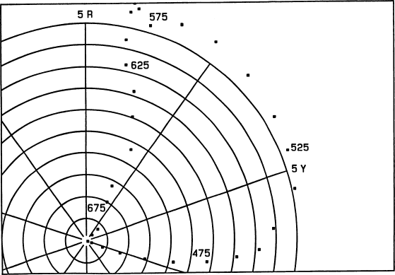
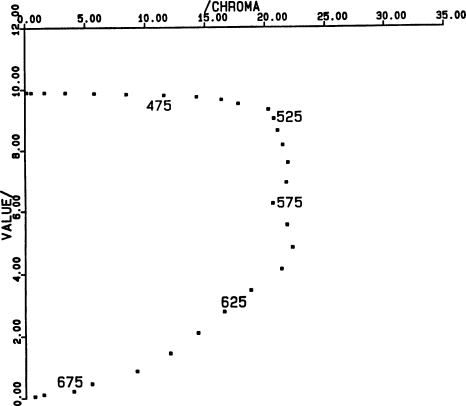
Fig. 4.
Colors of surfaces that are black at short wavelengths
and perfectly reflecting at wavelengths longer than that
of this reflectance step, plotted in the (hue, chroma) Munsell
subspace. Selected points are labelled with the wavelength
(in nanometers) at which the spectral jump occurs. The next
figure shows the missing coordinate.
 However, the “blue” channel contributes practically
nothing to the sensation of brightness, and hence nothing
to the Y integral. Consequently, the apparent lightness of
such a hypothetical surface is hardly decreased until the
transition wavelength reaches about 500 nm, where the Y
integral begins to decrease (see Fig. 5). Furthermore, until
it does, the green/red ratio remains nearly constant. Thus,
all such surfaces, with a step in the spectrum between 400
and 500 nm, have very nearly the same dominant wavelength
and very nearly the same hue (near 3 GY). Only the purity (in
stimulus terms) or chroma (in perceptual terms) changes as
the step moves to longer wavelengths.
However, the “blue” channel contributes practically
nothing to the sensation of brightness, and hence nothing
to the Y integral. Consequently, the apparent lightness of
such a hypothetical surface is hardly decreased until the
transition wavelength reaches about 500 nm, where the Y
integral begins to decrease (see Fig. 5). Furthermore, until
it does, the green/red ratio remains nearly constant. Thus,
all such surfaces, with a step in the spectrum between 400
and 500 nm, have very nearly the same dominant wavelength
and very nearly the same hue (near 3 GY). Only the purity (in
stimulus terms) or chroma (in perceptual terms) changes as
the step moves to longer wavelengths.
Fig. 5.
Colors of surfaces that are black at short wavelengths
and perfectly reflecting at wavelengths longer than that
of this reflectance step, plotted in the (chroma, value)
Munsell subspace. Selected points are labelled with the
wavelength at which the spectral jump occurs. The previous
figure shows the missing coordinate.
As the step moves past 500 nm, the Y integral begins to
decrease. The surface becomes darker and redder. The
excitation purity is nearly 100% for all these colors. The
dominant wavelength passes through a region in which the
eye is remarkably sensitive to small changes; for example,
saturated colors of Munsell hues 2.5 Y and 10 YR differ in
dominant wavelength by only about 2.7 nm, corresponding to
motion of the step from 531 to 539 nm (see Fig. 4). An
experienced observer can distinguish ten hues in this range.
In fact, over the whole range of “yellow” Munsell hues,
from 10 YR (= 0Y) to 10Y, the dominant wavelength of
saturated colors changes only 10 nm, corresponding to
displacement of the spectral step from 501 to 539 nm. Thus,
the very obvious change of 2.5 Munsell hue steps from one
page of the Munsell book to the next corresponds, on the
average, to less than 10 nm in the step wavelength, or 2.5
nm in the dominant wavelength.
This is comparable to the spread in half-peak wavelengths
among the Io spectra within each individual color class
on Fig. 4 of Soderblom et al. (1980): nominally similar
regions on Io have, in fact, colors that are readily perceived
to be very different by a color-normal observer. Human
color vision makes finer distinctions among surfaces with
such reflectance spectra than Soderblom et al. (1980)
considered significant. Thus, a quantitative color
specification, such as a Munsell renotation, actually
contains more detailed information about such surfaces
than the Voyager TV data can reliably supply.
 Indeed, normal color perception is so sensitive to
small differences in spectral reflectance among yellow
surfaces that such surfaces may be more readily
distinguished by their colors than by plotting their
spectra. Fig. 6 shows reflectance spectra of two rather
similar yellow surfaces that differ by one Munsell hue
unit. The eye can distinguish hue differences of about 1/4
hue step between such saturated colors. Thus, about 3 more
equally-spaced colors could be interpolated between these;
but it would be difficult to draw another three distinctly
different curves between those shown in Fig. 6.
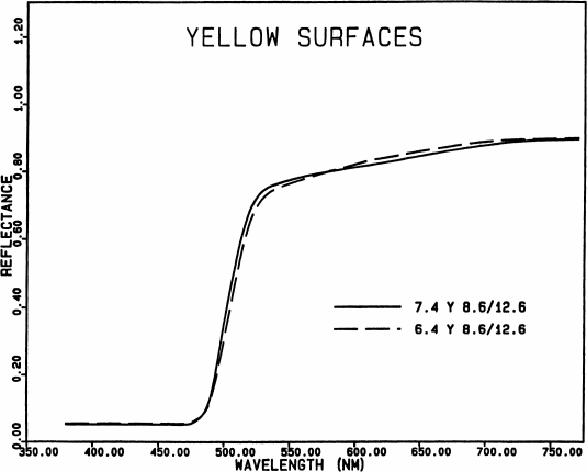
Indeed, normal color perception is so sensitive to
small differences in spectral reflectance among yellow
surfaces that such surfaces may be more readily
distinguished by their colors than by plotting their
spectra. Fig. 6 shows reflectance spectra of two rather
similar yellow surfaces that differ by one Munsell hue
unit. The eye can distinguish hue differences of about 1/4
hue step between such saturated colors. Thus, about 3 more
equally-spaced colors could be interpolated between these;
but it would be difficult to draw another three distinctly
different curves between those shown in Fig. 6.
Fig. 6.
Spectral reflectance curves of two similar yellow
surfaces. The eye can distinguish color differences about
1/4 as large as that between these two surfaces.
This extreme sensitivity accounts for the narrowness
of the part of a spectrum that appears yellow. It also
accounts for the difficulty in reproducing such colors
accurately on the printed page, and for the very large hue
shifts produced by the Voyager TV team by reproducing
pictures a few dozen nanometers to the red of the bands in
which they were taken.
The remarkably different character of the perceived
changes as the step passes 500 nm, from mainly a change in
chroma at nearly constant hue and brightness (on the short
wavelength side of 500 nm) to large changes in hue and
brightness at nearly constant chroma (on the long wavelength
side), is due to the strong overlap of the spectral
sensitivities of the red and green cones, on the one hand,
compared to their very small overlap with the response
curve of the blue cones, on the other. For steps below 500 nm,
only the blue/yellow channel of color vision is strongly
affected by step position. For longer step wavelengths,
this channel is forced to its yellow extreme, and both the
red/green and black/white channels are sensitive to the
wavelength at the step.
8 NONLINEARITY AND COLOR NAMING
Because the red and green cones have so nearly the same
spectral responses, the red-green opponent mechanism
cancels much of their common response and makes small
nonlinear differences between the red and green channels
easily visible in the yellowish hues. For example, the
green content of the greenish yellows is hardly visible
at high Munsell value, but adding a small amount of gray or
black to them makes the green stand out prominently. A
moderate yellow like Munsell 5Y 7/7 appears moderate olive
if its reflectance is reduced 5 or 10 times, to 5Y 3/7.
Likewise, 8Y 9/2.5 is just pale yellow, but 8Y 4/2.5 is
grayish olive (Kelly and Judd, 1976). I have pointed out
elsewhere (Young, 1984) these effects in the perceived
colors of Jupiter, which appears pale yellow when seen as
a bright light against black space, but looks olive when
seen with the much brighter Moon, which lowers the perceived
lightness of Jupiter.
Furthermore, a pale orange yellow like 7.5 YR 9/4 looks
pale yellowish pink when desaturated to 7.5 YR 9/2. At Munsell
hue 6YR, which is slightly to the yellow side of the purest
orange hues, all colors lighter than Munsell value 6.5 and
less saturated than chroma /6 are called yellowish pink,
brownish pink, or pinkish gray or white. Thus, although the
“pinks” dominate light colors on the purplish side of red
(near Munsell hue 2.5 R), an orange yellow will be called “pink”
if it is sufficiently light and unsaturated.
These effects help explain the pinkish color sometimes
attributed to Io by observers who see it next to greenish-
yellow Jupiter. Only a small change in the adaptation of
the eye, from white sunlight to the greenish yellow of
Jupiter, could shift Io's perceived hue from its actual pale
greenish yellow near Munsell 6Y to 8YR, the edge of the
yellowish pinks.
Furthermore, the red and brown colors often seen on
Jupiter itself are due to the well known expansion of the
range of perceived colors in a scene of limited color range.
For example, Hurvich and Jameson (1960) showed a complex
display of low-saturation yellowish greens, not very
different from the range of stimuli presented by Jupiter
and Io at the telescope, to seven observers in a laboratory
setting. The perceived hues included the pure red hue
Munsell 5R (see their Fig. 12). The lightest areas in the
same display were near Y=0.6 (Munsell value 8.1), but areas
only slightly darker with Y=0.4 (value 6.8) appeared as dark
as Y=0.1 (value 3.7; “brown” appears below value 6.5).
Thus, the human visual system considerably enhances low-
contrast images.
This exaggeration of the gamut of colors perceived in
a scene of very limited color range, such as Jupiter presents
at the telescope, probably accounts for the acceptance of
highly exaggerated false-color pictures as realistic by
the Voyager imaging team. Although, as Smith is reported
(Goldberg, 1979) to have said, “That is what Jupiter looks
like to the eye”, it is not what Jupiter would look like if
we could see it in a normal terrestrial scene with a full
range of colors.
9 IO
The reflectance spectrum of Io is well known, both
globally from ground-based spectrophotometry, and locally
from Voyager TV measurements through filters. It is marked
by a great deficiency of what Newton called violet and
indigo rays, being rather flat at longer wavelengths. The
procedure described above was applied to the Io spectra
by Young (1984); the resulting colors were pale, grayish,
and somewhat greenish yellows, in the NBS-ISCC naming system.
 Newton (1730; p.164) found that “the mixture of all Colours
but violet and indigo will compound a faint yellow, verging
more to green than to orange.” This describes exactly both
the reflectance spectrum and the color of Io (Young, 1984,
1985). He continues, “Thus it is by the computation: And
they that please to view the Colours … will find it so in
Nature.”
Newton (1730; p.164) found that “the mixture of all Colours
but violet and indigo will compound a faint yellow, verging
more to green than to orange.” This describes exactly both
the reflectance spectrum and the color of Io (Young, 1984,
1985). He continues, “Thus it is by the computation: And
they that please to view the Colours … will find it so in
Nature.”
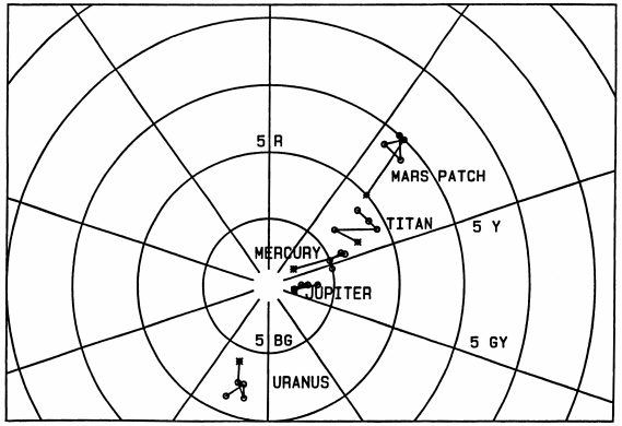
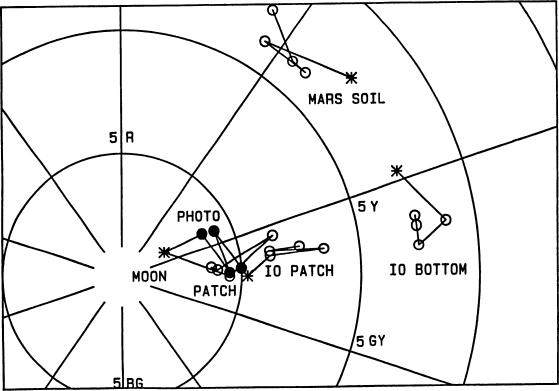
Fig. 7.
Planetary target colors (asterisks) and colors
actually printed (open symbols) as square patches in the
text on pp. 401-402 of Young (1985). Target and actual
colors for each object are connected by straight lines.
The target colors were calculated from published planetary
reflectance spectra, and the printed colors were determined
by comparison with the Munsell Book of Color; the
uncertainties in these estimates are about the size of
the plotted symbols. The deviation of the symbols for each
object from the target color gives some idea of the accuracy
with which colors can be reproduced in careful press work,
and their scatter indicates the precision of color printing.
This figure shows the Munsell (hue, chroma) subspace; Fig. 8
shows the missing coordinate.
So said Newton; and so say I. They that please to view
the colors will find them closely represented in Young
(1985). How closely? Figs. 7–12 compare the target colors
(asterisks) with those that were actually printed (circles)
in four different parts of the press run. The symbol size
in these diagrams is comparable to the precision of visual
color matches in each dimension. As these diagrams use
Munsell (i.e., perceived color) coordinates rather than
chromaticity (i.e., stimulus) coordinates, they are
approximately perceptually uniform.
 While most of the planetary colors published in
(Young, 1985) were fairly close to the actual planetary
colors, Mars was appreciably too red. Figs. 7
and 8 show that
the true color of Mars is intermediate between the printed
colors of the “Mars” color patch and the
“Titan” patch; if
anything, the latter is closer to the color of Mars. This,
with the excessive saturation of the colors printed for
the Moon and Mercury, was due to the difficulties of the
printing process. It is not possible to print colors with
very high accuracy, as one sees from the separation of the
printed colors from their targets, nor with very high
precision, as one sees from the scatter among the four
samples.
While most of the planetary colors published in
(Young, 1985) were fairly close to the actual planetary
colors, Mars was appreciably too red. Figs. 7
and 8 show that
the true color of Mars is intermediate between the printed
colors of the “Mars” color patch and the
“Titan” patch; if
anything, the latter is closer to the color of Mars. This,
with the excessive saturation of the colors printed for
the Moon and Mercury, was due to the difficulties of the
printing process. It is not possible to print colors with
very high accuracy, as one sees from the separation of the
printed colors from their targets, nor with very high
precision, as one sees from the scatter among the four
samples.
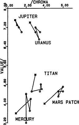
Fig. 8.
Munsell (chroma, value) subspace for the colors shown
in Fig. 7.
 The Io picture at the top of p.400 (Young, 1985) was about
the correct hue (see Fig. 11);
the picture at the bottom of
the page was slightly too green (see Fig. 9). As both
ground-based and Voyager pictures show, the belts of Jupiter
are similar in color to the average color of Io, and hence
considerably less saturated than the top Io picture, which
includes one of the most saturated areas on Io. Although
Jupiter's bright zones were reproduced correctly, the belts
were much too red and too dark, even in the low-contrast
version.
The Io picture at the top of p.400 (Young, 1985) was about
the correct hue (see Fig. 11);
the picture at the bottom of
the page was slightly too green (see Fig. 9). As both
ground-based and Voyager pictures show, the belts of Jupiter
are similar in color to the average color of Io, and hence
considerably less saturated than the top Io picture, which
includes one of the most saturated areas on Io. Although
Jupiter's bright zones were reproduced correctly, the belts
were much too red and too dark, even in the low-contrast
version.
Fig. 9.
Additional colors from (Young, 1985), as shown in
Fig. 7; see Fig. 10 for the missing coordinate. The “Io
patch” appears on p. 402 of (Young, 1985); “Io bottom”
refers to the most saturated portion of the Io picture at
the bottom of p. 400. The “Moon photo” (filled symbols)
is on p. 399, and the “Moon patch” (open symbols) is on
p. 401. “Mars soil” refers to the picture at the top of p. 401.
It is unfortunate that no really true color picture
of Jupiter has ever been published from Voyager data.
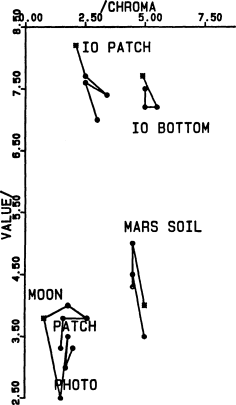
Fig. 10 (left).
Munsell (chroma, value) subspace for the colors
shown in Fig. 9.
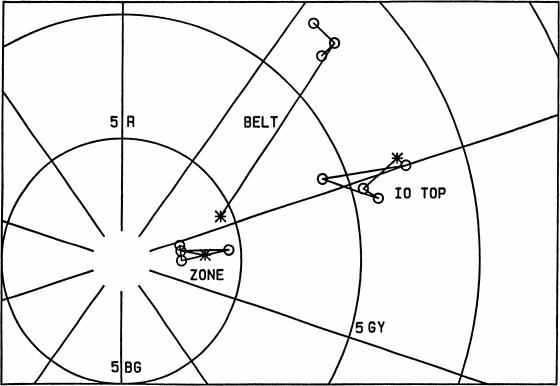
Fig. 11 (right).
Additional colors from (Young, 1985), as shown in
Fig. 7; see Fig. 12 for the missing coordinate. “Io top” is
a saturated area in the picture at the top of p. 400 of
(Young, 1985); “Belt” and “Zone” refer to
the lower-contrast
panel of the Jupiter picture on p. 402. Note that the contrast
of this picture is still unrealistically high: the belt
was reproduced with nearly 3 times more chroma and much
redder than spectrophotometry of Jupiter indicates. The
true color of belts on Jupiter is very similar to the average
color of Io, but slightly redder (i.e., nearly the same hue
as the Io picture at the top of p. 400, but with about half the
chroma of the most saturated areas in that picture).
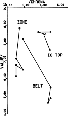
Fig. 12 (left).
Munsell (chroma, value) subspace for the colors
shown in Fig. 11.
10 HOMILETIC DISCUSSION
Color is so important a part of vision that we habitually
rely on it to identify materials, including those that may
occur on planetary surfaces; to distinguish between good
and unpleasant foods, as in rejecting “green” fruits; and
even to ensure our personal safety by means of colored
traffic signals and navigational lights. This sensation
not only “colors our language” but also our thinking; and
we can clarify both by understanding color well.
Planetary scientists are already accustomed to dealing
with interdisciplinary problems. If, to understand color,
we must acquaint ourselves with some unfamiliar branches
of science, this is hardly a new situation. And the reward
is well worth the effort, for we both receive and distribute
most of our information visually.
I have heard some scientists argue that “color isn't
important”, and that “all the science is in the numbers”.
(If they really believed that, they would not show color
slides at DPS meetings!) This is a naive attitude; color
does
influence our thinking, whether we recognize it or not.
The enormous importance of color was recognised by the
award of the 1908 Nobel prize in physics to G. J. Lippmann for
his development of a method of color photography so
imperfect it is now almost forgotten. To ignore the
importance of color is to risk being led astray by incorrect
colors. At the Workshop on Volcanic Flows on Io, there were
gasps of amazement when the customary false-color Voyager
pictures were replaced by more accurately colored ones,
and one scientist said he would have done his work
differently if he had seen the correct colors earlier.
Not only will we be less likely to deceive ourselves
with falsely colored pictures, but we may prevent a
public-relations fiasco in dealing with a public that can
be resentful at being misled, and that supports our efforts
with its taxes. Accurately colored pictures are one thing
the public definitely expects of us, and are by far the
most accessible product we can produce for the
scientifically untrained layman. Neglecting color could
be hazardous to the health of the whole planetary research
program.
Let me recall a few words of Tim Mutch (1978), who wrote,
“we had no intimation of the immediate and widespread
public interest in the first color products.” He went on
to describe the steps that led to publication of pictures
of Mars with a blue sky. “Several days after the first release,
we distributed a second version, this time with the sky
reddish. Predictably, newspaper headlines of 'Martian sky
turns from blue to red' were followed by accounts of
scientific fallibility. We smiled painfully when reporters
asked us if the sky would turn green in a subsequent version.”
I had hoped that the lessons of Viking had been learned.
To quote Tim Mutch again, “we were dismally unprepared to
reconstruct and analyze the first color picture. … we
failed to appreciate … many subtle problems which,
uncorrected, could produce major changes in color.” This
seems to remain true.
11 APPENDIX A
The precision of visual color matching was investigated
by MacAdam (1942) in a classic paper. His results of most
interest to the planetary scientist are those for neutral
and slightly yellowish colors, corresponding to those
that commonly occur on planets. The chromaticity of the
point closest to Illuminant C was (x, y) = (0.305, 0.323),
at which the long semiaxis of the ellipse that represents
the standard deviation of visual color matches was 0.0023,
and the short semiaxis was 0.0009 in length. For the nearby
point at (0.385, 0.393), corresponding to light yellow
surfaces, the semiaxes were 0.0038 and 0.0016; in both
cases, the major axis lay nearly in the direction of
increasing yellow saturation.
We may compare these values for the eye's sensitivity
to small color differences to that of broadband
photoelectric photometry in the UBV system. Many planetary
and mineral surfaces have a nearly linear variation of
reflectance with wavelength, as discussed in the text; so
we may ask what slope change in the reflectance of a nearly
neutral gray surface is detectable to either the eye or
the photometer.
If we adopt 441.5 nm and 550 nm as the effective wave-
lengths of the B and V passbands, a slope in reflectance of
0.00848%/nm will make the (B - V) color index of the
reflected light 0.01 mag redder than that of the Sun. This
is comparable to or less than the smallest difference in
(B − V) usually detectable in a single observation. For
example, FitzGerald (1973) found a standard deviation of
0.011 mag in (B − V) in comparing a number of catalogs; and
the errors given by Johnson and Harris (1954) for the
original UBV standard stars correspond to 0.02 mag per
observation in (B − V).
The slope of 0.00848%/nm required to produce a change
of 0.01 in the (B − V) color index produces a surface with
chromaticity coordinates x = 0.3124, y = 0.3182 under
Illuminant C, corresponding to Munsell chroma /0.13, or an
excitation purity of about 1%. This point lies about 0.0030
units in (x, y) space from Illuminant C. According to
MacAdam (1942), the standard deviation of color matches in
this region of color space is at worst 0.0023, in about the
direction this point lies from Illuminant C.
In other words, a spectral slope change that alters
(B − V) by 0.01 mag differs from a flat spectrum by
0.0030/0.0023 = 1.3 times the standard deviation of visual
color matches, although it is a little less than the standard
deviation of (B − V) color-index measurements. This is
consistent with MacAdam's statement that the first visually
detectable step from white corresponds to 0.2 to 0.7%
excitation purity, depending on the wavelength. The eye
is thus about twice as precise in detecting small changes
in spectral slope of a low-saturation surface as is UBV
photoelectric photometry.
When we consider that the eye's error is only 0.0009
or less than half as large in the orthogonal direction
(roughly that of hue), it becomes even clearer that the eye
is more precise than UBV photometry for detecting small
color differences among nearly neutral or pale yellowish
surfaces, such as are typical of planets and satellites.
Indeed, the situation is even worse for UBV photometry
than I have represented here; for the above figures for
this popular system refer only to the precision reached
in comparing normal stellar spectra with one another. But
the spectral energy distributions of planets are unlike
those of stars, and in fact the UBV system is not well defined
for many solar-system objects.
Thus, for example, we cannot place Mars on this system
with more precision than a tenth of a magnitude in any band
or color index of the UBV system (Young, 1974b). But normal
human eyes are made to tighter tolerances than we can make
UBV photometers; furthermore, the overlapping response
functions of the visual pigments produce much less aliasing
than do the UBV passbands. Consequently, two people with
normal color vision can agree on the color of Mars much
more closely than can two astronomers trying to measure
it with UBV photometers.
12 APPENDIX B
The FORTRAN 77 subroutine listed here converts spectral
reflectances, tabulated at 10-nm intervals, into CIE
chromaticity coordinates, assuming Illuminant C. The DATA
statements contain the CIE 1931 color-matching functions
weighted by the relative spectral radiant power
distribution for Illuminant C, taken from Table I(3.3.8) of
Wyszecki and Stiles (1982). These functions allow the
accurate approximation of the necessary integrals by the
trapezoidal rule.
Chapter 5 of MacAdam (1981) gives a very thorough
discussion of various numerical methods for calculating
the chromaticity coordinates (x, y) and luminance factor
(Y) for a surface of known spectral reflectance. The method
employed here is known in the color-science literature as
the method of weighted ordinates; see also p.159 of Wyszecki
and Stiles (1982).
This method was checked by Nickerson (1935), using the
spectrophotometric curves of the most saturated Munsell
papers of the 10 principal hues (5R, 5YR, 5Y, etc.) Fig. 1
of that paper shows that these curves have much steeper
sides than the reflectance curve of any known planetary
surface. Thus, the error committed in computing CIE
coordinates of the saturated Munsell hues will exceed
those for planets. Nickerson found that summation for 10
nm intervals, as employed here, “gives x and y with an average
uncertainty of 0.0004.” This value should be compared to the
smallest visually detectable chromaticity differences,
which are 0.001 or 0.002, according to MacAdam (1942).
These results were confirmed and extended by De Kerf
(1958), who found that the errors of this method were less
than the just-perceptible separation of colors for nearly
all surfaces, although somewhat larger errors were made
in computing the colors of interference filters and
didymium-glass filters, which had fine structure that was
not adequately sampled at 10 nm intervals. De Kerf
concluded that our method was “sufficiently accurate for
our purpose.”
The program has been checked in several ways. First,
a pure-white spectral reflectance, identically equal to
unity, was run to verify that the known coordinates for
Illuminant C (x = 0.3101, y = 0.3163, Y = 100%) were produced.
Second, the colors of several paint samples whose
spectral reflectances had been measured by Parker Pace of
Frazee Paint and Wallcoverings (San Diego, Calif.) were first
estimated by direct comparison with the Munsell color
standards, and then computed by running the tabulated
reflectance spectra through the program, and converting
the resulting chromaticity coordinates into a Munsell
renotation, as described in the text. The agreement was
within the accuracy of the estimates from the Munsell book.
Third, spectral reflectance data with Munsell notations
and chromaticity coordinates for several paints produced
by Nuodex, Inc. (Piscataway, N.J.) were provided by Dr. Dan Phillips.
One of these that is very similar to the most saturated
regions on Io was run through the program listed here. The
computed chromaticity coordinates deviated by an average
of one part in ten thousand from those computed at Nuodex.
As the tabulated data extend only from 400 to 700 nm, I believe
the error is non-zero because of differences in
extrapolating the spectra to the full 380 – 770 nm interval.
Fourth, a crude check can be obtained by comparing
the computed Io color against the observations of careful
observers. Probably the most intensive visual observations
of the Galilean satellites were made by Lyot and his
co-workers Gentili and Camichel when they mapped the
satellites at Pic du Midi (Lyot 1943, 1953). Observations
were made in 1941 with a 38 cm aperture, and “With the 500
enlargement … the satellites appeared as disks with very
sharp edges and each of them could be identified very
easily by its diameter, its brightness, and its color … .
Io, notably larger than Europa, was more pale and of a
yellowish color. … Ganymede, comparable to Io in color and
brightness, surpassed all the other satellites in diameter.”
In 1943 and 1944, these observations were repeated
with an aperture of 60 cm, which should make colors more
visible. Lyot (1953) reported that Io “looked like a little
disk of a light yellow color,” and that Ganymede “is slightly
yellow, like Io.” My earlier determination of the color of
Io from ground-based spectrophotometry (Young, 1984) was
near the boundary between “pale yellow green” and “pale
yellow”, in the ISCC-NBS color naming system. As objects seen
through a telescope are perceived more nearly in aperture
mode, as colored lights, than as surfaces, thereby losing
their gray content, one should expect the greenish tint
of Io to be less perceptible telescopically. Simultaneous
contrast with the greenish tint of Jupiter may also make
Io appear less green. On the whole, I believe the agreement
is as good as can be expected.
Taking all the checks into consideration, I believe
there is negligible chance of any appreciable error in
colors determined from spectrophotometric data by using
this program and the standard methods described in the text.
           SUBROUTINE CIE (REFL, X,Y,BIGY)
     C
     C  INPUT IS SPECTRAL REFLECTANCE TABLE (REFL);
     C
     C  RETURNS VALUES OF CIE CHROMATICITY COORDINATES (X, Y)
     C   AND VISUAL REFLECTANCE (BIGY) FOR ILLUMINANT C.
     C
     C  REFLECTANCE DATA ARE STORED AT 10 NM INTERVALS, WITH
     C  REFL(1)  = REFLECTANCE AT 380 NM, AND
     C  REFL(40) = REFLECTANCE AT 770 NM.
     C
           DIMENSION XBAR(40),YBAR(40),ZBAR(40),REFL(40)
     C
     C   WEIGHTS INCLUDE ILLUMINANT C; SEE TABLE I(3.3.8) OF
     C   WYSZECKI & STILES (1982), P.768.
     C
           DATA XBAR/.004,.019,.085,.329,1.238,2.997,3.975,3.915,3.362,
          1 2.272,1.112,.363,.052,.089,.576,1.523,2.785,4.282,5.88,7.322,
          2 8.417,8.984,8.949,8.325,7.07,5.309,3.693,2.349,1.361,.708,
          3 .369,.171,.082,.039,.019,.008,.004,.002,.001,.001/
           DATA YBAR/.0,.0,.002,.009,.037,.122,.262,.443,.694,1.058,1.618,
          1 2.358,3.401,4.833,6.462,7.934,9.149,9.832,9.841,9.147,7.992,
          2 6.627,5.316,4.176,3.153,2.19,1.443,.886,.504,.259,.134,.062,
          3 .029,.014,.006,.003,.002,.001,.001,0./
           DATA ZBAR/.02,.089,.404,1.57,5.949,14.628,19.938,20.638,19.299,
          1 14.972,9.461,5.274,2.864,1.52,.712,.388,.195,.086,.039,.02,
          2 .016,.01,.007,.002,.002,0.,0.,0.,0.,0.,0.,0.,0.,0.,0.,0.,0.,
          3 0.,0.,0./
     C
           X=0.
           Y=0.
           Z=0.
               C  USE SUMS FOR INTEGRALS.
           DO 20 I=1,40
           X=X+REFL(I)*XBAR(I)
           Y=Y+REFL(I)*YBAR(I)
                  20 Z=Z+REFL(I)*ZBAR(I)
           BIGY=Y
           SUM=X+Y+Z
           X=X/SUM
           Y=Y/SUM
           RETURN
           END
13 ACKNOWLEDGMENTS
This work was supported by Planetary Atmospheres
Grant NAGW-250 from the National Aeronautics and Space
Administration. Heidi Hammel kindly loaned me her copy of
Sky & Telescope for color checking. I thank Joe Boyce for
arranging special travel to the Io Volcanic Flows Workshop,
and for encouraging me to discuss the broader implications
of color in the planetary literature. This paper is in
response to a request for a short explanation of color by
the Workshop.
14 REFERENCES
Birren, F. (1969). A Grammar of Color. Van Nostrand
Reinhold, New York.
Boynton, R. M. (1979). Human Color Vision. Holt, Rinehart
and Winston, New York.
Committee on Colorimetry, Optical Society of
America (1963). The Science of Color. Optical
Society of America, Washington, DC.
D'Zmura, M., and P. Lennie (1986). Mechanisms of color
constancy. J. Opt. Soc. Amer. A 3, 1662-1672.
De Kerf, J. L. F. (1958). Accuracy of tristimulus
computations. J. Opt. Soc. Amer. 48, 334-338.
Derrington, A. M., J. Krauskopf, and P. Lennie (1984).
Chromatic mechanisms in lateral geniculate
nucleus of Macaque. J. Physiol. 357, 241-265.
FitzGerald, M. P. (1973). Error analysis of the
photoelectric catalogue. Astron. Astrophys.
Suppl. 9, 297-311.
Goldberg, N. (1979). Jupiter close up. Popular
Photography 85 (3), 82-126.
Henbest, N., and M. Marten (1983). The New Astronomy, pp. 28-29.
Cambridge University Press, Cambridge.
Huck, F. O., D. J. Jobson, S. K. Park, S. D. Wall, R. E. Arvidson,
W. R. Patterson, and W. D. Benton (1977).
Spectrophotometric and color estimates of the
Viking lander sites. J. Geophys. Res. 82, 4401-4411.
Hunt, G., and P. Moore (1981). Jupiter, p. 60. Rand McNally,
New York.
Hurvich, L. M., and D. Jameson (1960). Perceived color,
induction effects, and opponent-response
mechanisms. J. Gen. Physiol. 43 (6) Suppl. 2, 63-80.
Johnson, H. L., and D. L. Harris III (1954). Three-color
observations of 108 stars intended for use as
photometric standards. Astrophys. J. 120, 196-199.
Kelly, K. L. (1943). Color designations for lights. J.
Opt. Soc. Amer. 33, 627-632.
Kelly, K. L., and D. B. Judd (1976). Color: Universal
Language and Dictionary of Names (NBS Special
Publication 440). National Bureau of Standards,
Washington, D. C.
Krauskopf, J., D. R. Williams, and D. W. Heeley (1982).
Cardinal directions of color space. Vision Res.
22, 1123-1131.
Kuehni, R. G. (1983). Color — Essence and Logic. Van
Nostrand Reinhold, New York.
Le Grand, Y. (1957). Light, Colour, and Vision, p. 220.
John Wiley, New York.
Lee, Hsien-Che (1986). Method for computing the
scene-illuminant chromaticity from specular
highlights. J. Opt. Soc. Amer. A 3, 1694-1699.
Lyot, B. (1943). Observations planetaires au Pic du
Midi, en 1941. L'Astronomie 57, 49-60.
Lyot, B. (1953). l'Aspect des planetes au Pic du Midi
dans une lunette de 60 cm d'ouverture.
L'Astronomie 67, 3-21.
MacAdam, D. L. (1942). Visual sensitivities to color
differences in daylight. J. Opt. Soc. Amer. 32, 247-274.
MacAdam, D. L. (1981). Color Measurement: Theme and
Variations. Springer-Verlag, Berlin.
Malin, D., and P. Murdin (1984). Colours of the Stars.
Cambridge University Press, New York.
Maloney, L. T. (1986). Evaluation of linear models of
surface spectral reflectance with small
numbers of parameters. J. Opt. Soc. Amer. A 3, 1673-1683.
Morrison, Phil, Phylis Morrison, The Office of Charles
and Ray Eames (1982). Powers of Ten.
Scientific American Books, New York.
Mutch, T. A. (1978). “The Viking lander imaging
investigation: an anecdotal account” in The
Martian Landscape (NASA SP-425), p. 27. NASA, Washington, DC.
Newhall, S. M., D. Nickerson, and D. B. Judd (1943). Final
report of the O.S.A. subcommittee on the spacing
of the Munsell colors. J. Opt. Soc. Am. 33, 385-418.
Newton, I. (1730). Opticks: or, a Treatise of the
Reflections, Refractions, Inflections and
Colours of Light (4th Edition, 1730). Reprinted by
Dover Publications, Inc., New York, 1952.
Nickerson, D. (1935). Disk colorimetry; including a
comparison of methods for computing
tristimulus values for certain disks. J. Opt.
Soc. Amer. 25, 253-257.
Nickerson, D. (1947). Interrelation of color
specifications. Paper Trade J. 125, 153-171 = TAPPI
section 219-237.
Parkkinen, J., and T. Jaaskelainen (1987). Color
representation using statistical pattern
recognition. Appl. Opt. 26, 4240-4245.
Sill, G. (1973). Reflection spectra of solids of
planetary interest. Comm. Lunar Planet. Lab. 10, 1-7.
Smith, V. C., and J. Pokorny (1975). Spectral
sensitivity of the foveal cone photopigments
between 400 and 500 nm. Vis. Res. 15, 161-171.
Smith, B. A., L. A. Soderblom, T. V. Johnson, A. P.
Ingersoll, S. A. Collins, E. M. Shoemaker, G. E. Hunt, H.
Masursky, M. H. Carr, M. E. Davies, A. F. Cook II, J. Boyce, G.
E. Danielson, T. Owen, C. Sagan, R. F. Beebe, J. Veverka, R.
G. Strom, J. F. McCauley, D. Morrison, G. A. Briggs, and V.
E. Suomi (1979a). The Jupiter system through the
eyes of Voyager 1. Science 204, 951-972.
Smith, B. A., L. A. Soderblom, R. Beebe, J. Boyce, G. Briggs,
M. Carr, S. A. Collins, A. F. Cook II, G. E. Danielson, M. E.
Davies, G. E. Hunt, A. Ingersoll, T. V. Johnson, H.
Masursky, J. McCauley, D. Morrison, T. Owen, C. Sagan, E.
M. Shoemaker, R. Strom, V. E. Suomi, and J. Veverka
(1979b). The Galilean satellites and Jupiter:
Voyager 2 imaging science results. Science 206,
927-950.
Soderblom, L., T. Johnson, D. Morrison, E. Danielson, B.
Smith, J. Veverka, A. Cook, C. Sagan, P. Kupferman, D.
Pieri, J. Mosher, C. Avis, J. Gradie, and T. Clancy (1980).
Spectrophotometry of Io: Preliminary Voyager I
results. Geophys. Res. Lett. 7, 963-966.
Wyszecki, G., and W. S. Stiles (1982). Color Science; 2nd
Edition. John Wiley & Sons, New York.
Young, A. T. (1974a). Observational Technique and Data
Reduction. In Methods of Experimental Physics,
Vol. 12, Astrophysics, Part A: Optical and Infrared
(N. P. Carleton, Ed.), Chapter 3; see pp. 187-189.
Academic Press, New York.
Young, A. T. (1974b). UBV Photometry of Mars. In IAU
Symposium 65, Exploration of the Solar System
(A. Woszczyk and C. Iwaniszewska, Eds.), 253-285.
D. Reidel, Dordrecht.
Young, A. T. (1984). No sulfur flows on Io. Icarus 58, 197-226.
Young, A. T. (1985). What color is the solar system?.
Sky Tel. 69, 399-403.
File translated from
TEX
by
TTH,
version 2.92.
On 3 Nov 2004, 22:58.
HTML cleaned up manually by aty on
Thu Mar 10 12:29:38 PST 2005,
Fri Feb 10 20:33:59 PST 2006,
Wed Oct 25 18:51:08 PDT 2006,
and
Tue Apr 20 20:05:16 PDT 2021.
ALT tags added manually by aty on
Sat Mar 28 13:16:36 PDT 2009
The original version of this paper was the Final Report on NASA Planetary
Atmospheres Grant NAGW-250, which is available from the National Technical
Information Service at
ntrs.nasa.gov/archive/nasa/casi.ntrs.nasa.gov/19880009896_1988009896.pdf
Copyright © 2004 – 2009, 2012, 2021 Andrew T. Young