Ducted Mock-Mirage Simulations

Introduction

Here are the ducted mock-mirage simulations of my usual target.

Ducted mock mirages

The same model atmosphere, with a duct produced by a 2° inversion between 50 and 60 m, has been used for sunset simulations; so it's probably a good idea to use some of the same eye heights as were used for the sunsets. So I'll choose a height of 65 m, just a few meters above the top of the inversion (i.e., the top of the duct). (The sunset simulation for that height in this model is shown here.)

As usual, I'll start with the target just a few kilometers away, to show that there's no perceptible distortion at short ranges.

Nearby target: no distortion

So here's the target at 5 km, as seen from a height of 65 m. At this short range, the rays appear nearly straight, even in the inversion, which is shown shaded in these diagrams. So the transfer curve appears nearly straight; there's negligible distortion.

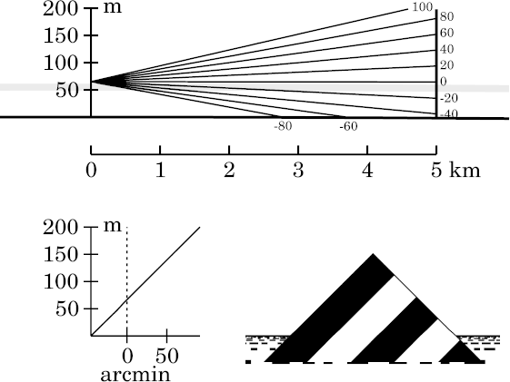
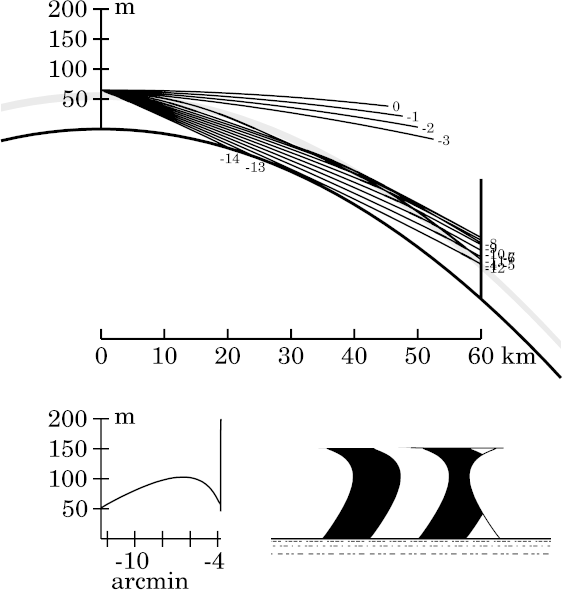
You can see that the target is much closer than the apparent “sea horizon”, both in the simulation at the right, and in the ray diagram above it. As usual, each ray is marked at its right-hand end with its altitude (in minutes of arc) at the observer.

Target at 15 km: distortion but no mirage

Here we see that strong refraction in the inversion layer has bent down the ray at −5′ apparent altitude at the observer. All the rays below it are also bent down, so that the lower part of the target is displaced upward, but not strongly deformed.

The upper part of the target, above the inversion, is seen through air with the standard lapse rate. So it's neither strongly displaced nor distorted.

However, the part of the target within the inversion layer is squashed together into a very thin interval of apparent altitude. That's the part between 50 and 60 m height, or the 5% of the 200 m-high target between 25% and 30% of its total height — see the little nearly-vertical piece of the transfer curve. So this zone of the target displays the effect called stooping (i.e., vertical compression).

This is an obvious consequence of the continuity of the image: the top is hardly displaced, while the bottom is raised; so the part in between has to be compressed.

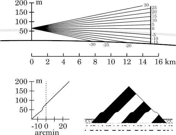
Target at 30 km: a transition at the horizon

At 30 km, the target is close to the apparent horizon. Now its distortions become more complex. In addition to the squashed zone, there's a zone of vertical stretching, or towering.

First, note that the stooped zone (the vertical section of the transfer curve) is now much larger. This is the platform-like feature in the simulated image, produced by the much larger deflection of rays near the top of the duct. (Look at the big gap that has developed at the target between the rays the observer sees at altitudes of −2′ and −4′.)

But just below this, at about −5′, there's a zone where the sloping side of the target is imaged as a vertical line (the short horizontal feature in the transfer curve). If you look at the ray diagram, that's caused by the convergence of the rays at −4′ and −6′ at the target: a tiny piece of the target has been expanded to this 2′ interval in the image.

Target at 40 km: a ducted mock mirage

At 40 km, the target is well beyond the apparent horizon. And here we clearly see an inverted image, produced by the ray-crossing near 34 km, where the ray at −6′ altitude at the observer crosses the one at −4′.

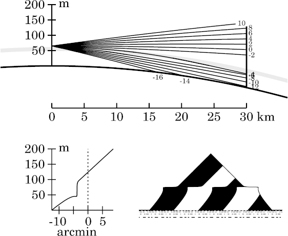
In the transfer curve, the flat spot near −5′ in the previous example has become a local maximum, so that features on the target near 50 m height are now seen at two different apparent altitudes: an erect image below, and inverted image above.

This appears to be a two-image mirage, with a discontinuity at the flat part of the image, between the inverted section seen at the top of the duct and the undistorted top above it. Actually, there is a third, erect image, so strongly compressed as to be effectively invisible, at this altitude, because of the vertical segment in the transfer plot. Whether or not there really is a discontinuity here depends on whether or not the lapse rate (rather than the temperature profile) is continuous.

The mock mirage here is not well developed; only about 1′ of the image is inverted. This might escape notice with the naked eye.

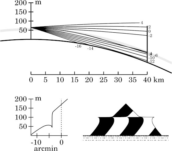
Target at 60 km: strong ducted mock mirage

As the target recedes, the inverted (miraged) part of the image becomes more dominant, as does the stooped part near −4′ altitude. The lowest parts of the target are disappearing behind the curve of the Earth.

Here, at 60 km, the whole upper section of the target has been stooped down nearly into a line above the miraged part. The 2-image character of the mirage is now more evident.

Note that more than 2′ of the image is now inverted. This would certainly be visible to the naked eye.

Also, notice that the upper part of the inverted image is vertically compressed, compared to the erect portion below it (look at the slopes of the sides). Of course, the lower part is vertically stretched, where it joins the erect section — just as at the fold line in the inferior mirage.

Back to the . . .
introduction to mock-mirage simulations

or the introduction to all mirage simulations

or the main mirage page

or the GF home page

or the website overview page