

Just as any well-behaved function of one variable can be represented as a sum of many sinusoidal components, a two-dimensional distribution (such as the brightness in an image, as a functions of the x and y coordinates) can also be represented as a sum of sinusoidal components. The main difference is that these components have an orientation (i.e., a direction) as well as a frequency.


Here you see pictures of two such components whose spatial frequencies have the same magnitude, but different directions:
The sinusoidal grating on the left varies only in the x direction;
the one on the right varies only in the y direction.
(We can also have gratings that vary along other, oblique directions; but
they're more tedious to draw.)


On the other hand, here are two spatial-frequency components with the same orientation, but different magnitudes. The frequency of the one on the left is 3 times higher than that of the one on the right.
(Actually, I've used the same image here twice, but told your browser to
squeeze it together in the left-hand picture, and expand it on the right.)
The examples above are what might be called monochromatic gratings: they have a single spatial frequency. But it's more useful to show a range of frequency in a single picture. Here's an example of a grating whose frequency increases linearly from left to right:

I hope these are enough to convey the general idea of spatial frequencies. Now, let's do some blurring, and then try to undo it.
To begin with, let's take that frequency ramp and smear it with a Gaussian blur, with a width of 10 pixels. Here's what we get:

You see that the low frequencies (at the left) are hardly affected; but the high frequencies, on the right, have practically disappeared. The effect of blurring is to attenuate the high spatial frequencies.
The mathematical operation of convolution corresponds to multiplying the Fourier transform of the original image with that of the convolution kernel; this product is the transform of the blurred image. So convolution (in ordinary space) corresponds to multiplying the various frequency components of the image by a filter function (in frequency space).
So the filter function of the blurring is the ratio of the Fourier transforms of the output and input images, as a function of spatial frequency. And this filter function is just the Fourier transform of the Gaussian kernel we used to do the blurring. As the Fourier transform of a Gaussian is also Gaussian in shape, we have a Gaussian filter here.
Before we try to un-blur the blurred image, let's try applying various sharpening filters to the original low-contrast frequency ramp shown above, to see what their filtering effects really are. As I'm a Linux user, I'll offer examples from the Gimp (the Gnu Image Manipulation Program); PhotoShop and other packages offer similar facilities.
![]() original
original
![]() 60
60
![]() 80
80
![]() 90
90
![]() 93
93
![]() 95
95
![]() 97
97
![]() original
original
There's moderate contrast enhancement at the higher frequencies, but it's not spectacular. And, at the higher enhancements (beyond about 90), there are clearly high-frequency artifacts introduced, at a scale of just one or two pixels. (There's also a lack of enhancement at the very edges of the image, which are exaggerated in width here; the actual image strips are only 12 pixels wide, but have been expanded to 100 pixels for display.)
Clearly, this filter is an edge-sharpener. It appears to be combining the Laplacian (second spatial derivative) of the original image with the original, so that the “sharpness” is the percentage of Laplacian in the final image.
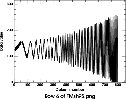 Here's a trace of a row from the middle of the 95%-sharpened image.
The parabolic increase in amplitude of the sinusoidal fringes with
increasing frequency (from left to right) is what you'd expect if the
second derivative is being added: differentiation of a sinusoid
multiplies it by the frequency, so a second derivative multiplies by
frequency squared .
Unfortunately, there is a lot of noise added to the lower frequencies, so this isn't a practical way to do a lot of high-pass filtering. (I'll explain the origin of that noise later.) And this much sharpening is already saturating a few of the highest-frequency fringes, at solid black and white.
A little thought shows that the smeared image is exactly the same as the original where the original has a constant brightness gradient in an area bigger than the Gaussian blurring kernel; this leaves the processed picture unchanged. It's only where the brightness gradient is changing that we get some effect.
So the Unsharp Mask operation, much like the Sharpen filter, basically adds the second spatial derivative of the picture to the original, making peaks higher and valleys deeper. Because each differentiation adds a factor of the frequency, this makes the filter function increase with the square of the frequency, at low spatial frequencies.
On the other hand, the blurred image has essentially constant gradients within areas smaller than the Gaussian convolution kernel. That means that all smaller (i.e., higher-frequency) details are amplified by practically the same amount. So the contrast enhancement of fine details becomes constant for features smaller than the blur size; the filter function levels off at high frequencies.
Let's look at the corresponding filter functions. The original image:


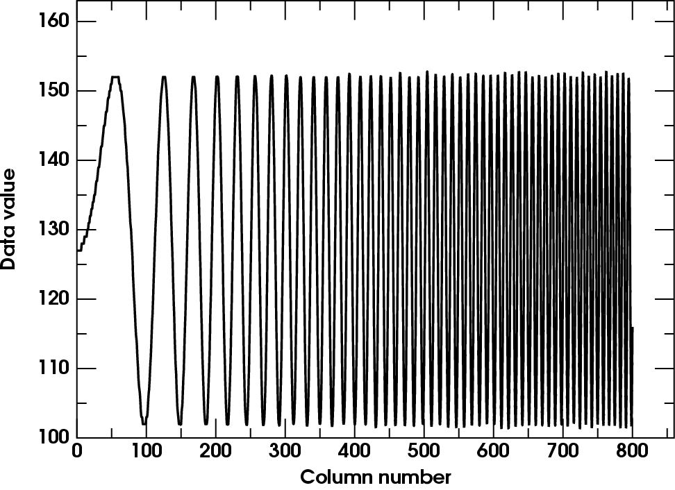
is compared here with a plot of its data values along a row. You can see
that (apart from a little sampling noise at the higher frequencies, where
some samples don't fall exactly at the extrema) the amplitude of the
original sinusoidal fringes is independent of frequency. Our input image
has a flat frequency spectrum.
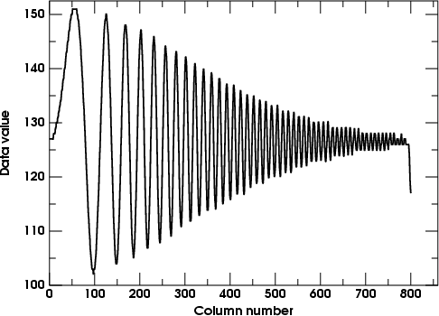 Now let's look at a row-trace of the blurred version. (It's displayed
here at half-scale; we don't need such a big plot as the one above.)
The little artifact at the right end can be ignored. It's a result of the way the Gaussian-blur module treats the edges of pictures: it reflects the image at the edge. As the original image was below the average level at the right-hand edge, the reflection of this low region has pulled the last few pixels down a bit.
As the Fourier transform of a Gaussian is just another Gaussian, we expect the filter function — which is just the amplitude of the envelope of the blurred image, in this case — will have that familiar bell-shape; and you see it does. (Only half of the bell shows here, of course; we don't try to show the negative frequencies, which would just be the reflection of this diagram about the vertical, zero-frequency, axis.) You can think of the filter as the upper envelope of this row-trace figure, if you just shift the horizontal axis up to the middle of the figure.
Now, bearing in mind the relation
between the Initial and Final images in the unsharp-masking process, we can easily see what the spatial filtering of the unsharp-masking operation must look like. The linearity of Fourier transforms allows us to interchange the order of operations: the sum of two transforms is the same as the transform of the sums of the original functions. So the differencing and adding of functions in the unsharp-masking operation corresponds to the same differencing and adding of their transforms, in frequency space.
So, as the frequency filter corresponding to a Gaussian blur also has that shape, the filter corresponding to the difference image is just (1 minus this Gaussian) — in other words, it's shaped like the lower envelope of the blurred-image row-trace above.
This makes the filter function of the Final image (the sum of the Initial and Difference images) go from 1 at low frequencies to 2 at high ones, if we use an “Amount” of 1. [If we use an Amount of 2, the high-frequency limit is 3; in general, the high frequencies saturate at a value that's 1 more than the Amount used, because of the (A + 1) factor in the equation above.]
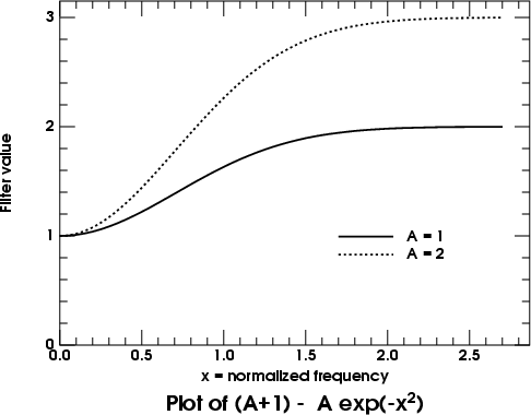 Mathematically, the Gaussian filter of the blurred image is something like
exp(−f2), where f is the spatial frequency (apart from a
frequency-scaling factor that's inversely proportional to the width of the
convolution kernel). So the filter function of the unsharp-mask operation
is something like
where A is the Amount. Here's a plot of this function, for A = 1 and 2.
Because the peak of a Gaussian is parabolic, the quadratic decrease of the Gaussian for small arguments explains the filter's quadratic increase at low frequencies. The sloping side of the (inverted) Gaussian produces the nearly linear filtering at intermediate frequencies (around column 300 in the row trace above); and the flat tail of the Gaussian accounts for the flat roll-over of the unsharp-mask filter at high frequencies.
The nearly linear part of the filter, where it has about half of its full (high-frequency) effect, occurs where the width of the Gaussian is about equal to the period of the sinusoidal fringes. In the above example, the Gaussian radius of 10 pixels means a diameter of 20; and the fringe spacing where the linear part occurs is also about 20 in the example above (around column 300).
Unfortunately, the people who wrote the Gimp's unsharp-mask routine adopted a different scaling convention for the radius of the blur; it turns out that you have to use a considerably smaller radius value in applying the UM enhancement to get the effect you'd expect from the remarks in the paragraph above: a radius of 2 or 3 in the UM enhancement corresponds to our blur of 10, above.
Some specific examples will help illustrate these effects. We'll start with our low-contrast sine-wave ramp, apply a few unsharp masks to it, and use row traces to illustrate the filter functions.
Here's the Unsharp Mask with radius 3 and amount 1. We expect the trace to look like (1 minus the Gaussian-blur filter) shown above. First, the unsharp-masked image:

And then its row-trace plot: —>
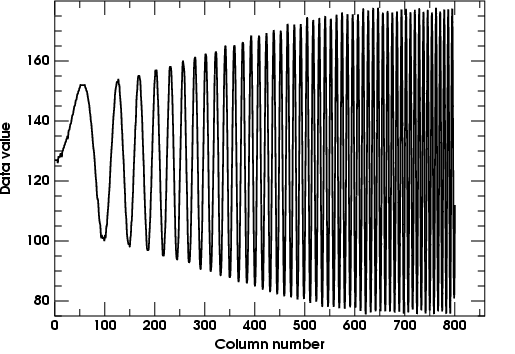
Notice that the amplitude of the high-frequency fringes is just about twice that at low frequencies, as we'd expect for A = 1. This nicely shows how the filter levels off at high frequencies; but it doesn't show the parabolic part at low frequencies well, because there are so few fringes visible at the left side.
To see the behavior at low frequencies, we must use a smaller radius. I'll
drop down to 1.0, just to emphasize the low-frequency region.

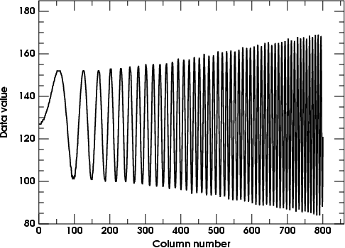 This shows the effect of unsharp masking with radius 1 and amount 1.0;
the parabolic start of the filter is well shown, but the frequency ramp
doesn't extend far enough to reach saturation.
The images don't look very different to the eye, apart from a little less contrast in the middle frequencies in the second case; but the numerical row traces clearly show the differences. And it's the numerical values we ultimately have to worry about.
These two examples show the effect of manipulating the Radius parameter of the unsharp-mask procedure. How about the Amount?
As this last example leaves plenty of room for contrast enhancement,
I'll keep the radius at 1.0 and raise the Amount to 4. The image below
shows the result.

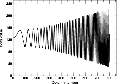 Now the enhancement at high frequencies is quite obvious. Notice that
the low frequencies remain almost unchanged.
The row-trace plot at the right shows the effect more quantitatively.
The parabolic increase at low frequencies becomes a more nearly linear
increase at high ones.
First, notice that the initial parabolic increase changes when the Radius value changes. As this is just the effect of adding a second derivative — or rather, a second difference , where Radius takes the place of a tabular interval — it is easy to see that doubling the Radius is like quadrupling the Amount, at low frequencies. In other words, the low-frequency increase of the unsharp-mask filter is just proportional to the product AR2.
Here's a comparison to illustrate that: first, the (Radius, Amount) combination (1, 4) that we just had above; and second, the combination (2, 1):

Radius = 1
Amount = 4

Radius = 2
Amount = 1
On the left side, these are almost exactly the same. But at the right, it's clear that the (1, 4) combination has much higher contrast at high frequencies than the (2, 1) setting. Obviously, that's because the former filter keeps increasing until it has raised the high-frequency contrast a factor of 5, while the latter levels off at 2. [Remember that the limiting factor is (A + 1), not just A.]
If you look closely, you'll see some slight differences between these two, even at low frequencies. While the average contrast of the low-frequency fringes is closely matched in the two cases, there are some faint high-frequency artifacts present in the (1, 4) case that are not visible in (2, 1).

Radius = 1
Amount = 5
There are clearly spurious fine stripes in the low-frequency fringes. So we can't keep increasing the Amount value indefinitely.
Where do these spurious features come from? Well, remember that all these images (including the Blurred image that's the intermediate step in the Unsharp Mask procedure) are stored to just 8-bit precision: a scale from 0 to 255. That means there are little jumps in the Difference image that are magnified when we multiply it by the Amount. A 1-bit discontinuity becomes 5 steps on the scale from 0 to 255 when it's multiplied by an Amount of 5. That's big enough to be visible.
What's happening here is that the high-pass filter is amplifying the little errors caused by limited precision. (Sometimes these errors are called digitizing noise, or “quantization” noise. As it varies randomly from one pixel to the next, it's a high-frequency component of the original image that's greatly enhanced by the Unsharp Mask filter.) This is very reminiscent of the high-frequency noise we saw in the Sharpen filter; indeed, it's exactly the same effect.
And we are starting with mathematically exact values. In a real-world image, there will be noise that may amount to several parts in 255 to begin with, even before amplification by the Amount.
Evidently, this is why the Gimp's “Amount” slider is limited to a value of 5.
We clearly can't use Amounts much larger than 5 before incurring unacceptable artifacts. This limits the amount of image restoration that can be done.
Here's what happens if you un-blur the blurred version with a Radius of 3 and an Amount of 1; the original (unblurred) image is shown just below the un-blurred one:

Blurred
version

Radius = 3
Amount = 1

Original
version
Well, that isn't very good. The unblurring worked pretty well at low frequencies, but was completely inadequate at high ones. That suggests that we should have tried a Radius of 2 instead of 3. Here's the result of trying that:

Blurred
version

Radius = 2
Amount = 1

Original
version
That's slightly worse; there's even less boost in the middle range. We forgot that the initial quadratic rise is proportional to AR2 — so lowering the radius lowered the rate of increase with frequency. So, let's try Radius = 2, Amount = 2:

Blurred
version

Radius = 2
Amount = 2

Original
version
That's clearly better, though those first few low-frequency fringes now seem a little too contrasty. But, as this seems to be going in the right direction, let's keep the low-frequency boost the same and extend the benefit to higher frequencies, by going to Radius = 1, Amount = 4:

Blurred
version

Radius = 1
Amount = 4

Original
version
Now it's plain that the low-frequency boost is a bit too large, while the high-frequency increase is still inadequate. And we clearly can't fiddle with things and improve the result much; this kind of discrepancy will always occur with the Unsharp Mask filter.
What's the problem? Can't we do any better?
(where x is a scaled spatial frequency); and its reciprocal is just
It may be useful to recall that
so that
which is the inverse of the Gaussian-blur filter.
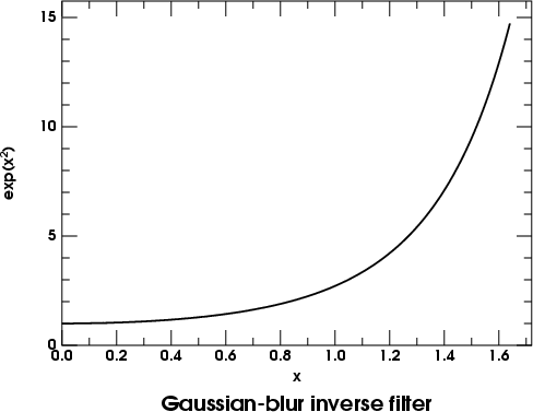 Here's a plot of that function. Instead of increasing quadratically at
first, and then flattening out (as the Unsharp-Mask filter does), it
increases quadratically and then goes shooting off towards infinity, ever
more steeply.
Clearly, we need something that becomes steeper than the initial quadratic increase; but the simple unsharp-mask filter becomes flatter instead. How can we get the increasing slope at high frequencies?
(Once again, x is a scaled frequency that allows for the radius of the Gaussian.) Expand the exponential, remembering that exp(−x) = 1 − x + ½x2 − … :
So the Unsharp Mask filter has the right quadratic term, if we choose A = 1, but the wrong sign for its fourth-power term. Is there any way to overcome this defect?
Even if we just apply the same UM filter twice, we see that some improvement is possible: the square of the UM(x) function given above is
If we choose A so as to make the coefficient of the x2 term unity, as in the desired inverse of the Gaussian, we get A = 1/2. This gives the squared filter the form
The fourth-power term still has the wrong sign, but it's only half as big as before.
As these functions are known exactly, it's preferable to determine the best-fit approximation in frequency space, rather than experiment with filters and images — which would require a trial-and-error search of a four-dimensional space, as there are four parameters to be determined: two Radius values, and two Amounts, for the two Unsharp Masks.
The only practical difficulty is that the product of two UM filters is extremely nonlinear in all four parameters. However, a good non-linear fitting program can handle the problem.
But there's a catch: if we try this blindly, allowing all the parameters to vary independently, we find that the radii tend toward zero, while the amounts march off toward infinity. What's happening is that the fitting tries to push the effect of that wrong-sign fourth-power term as far to the right as possible.
But we saw above that increasing the Amount beyond a modest value (on the order of 10) increases the digitizing noise unacceptably. So we need to limit the Amount of the combined filter.
where x = fR. If we had the product of two such functions, we would need to put subscripts on the A's and R's; but this is more complexity than we need to go into here.
To use this filter quantitatively, we need to understand its parameters better. The sharpness you specify in the Gimp's menu appears to be the percentage of the Laplacian in the final result. If we let S be the sharpness value (converted to a fraction from a percentage), that means that S is the fraction of Laplacian (proportional to frequency squared) in the final image, and that (1 − S) is the fraction of the original in the final result. The ratio of second-order to zero-order terms is therefore S/(1 − S) . This ought to be proportional to the product AR2 for the Unsharp Mask filter at low frequencies.
Before comparing the two types of filter, let's make sure that this interpretation of S is correct. If the amount of frequency-squared correction is indeed proportional to S/(1 − S) , we'd expect that applying the Sharpen filter twice would give an initial rise proportional to twice this [because (1 + x)2 = 1 + 2x + x2]. So applying an 80% sharpening twice should be nearly the same, at low frequencies, as applying a 90% sharpening once.
Here's the comparison of these two processes. The upper image is the frequency ramp, sharpened by 80% twice. The middle image is the ramp, sharpened by 90% just once. And the bottom image is the original, unsharpened frequency ramp.
![]() sh80 twice
sh80 twice
![]() sh90
sh90
![]() original
original
We see that indeed the low- and mid-frequency enhancements are similar, though of course the upper image is more contrasty at high frequencies, because the double sharpening has introduced a positive term proportional to the fourth power of the frequency — which is just what we need for the inverse of the Gaussian blur!
Recalling that the inverse of the Gaussian filter was just
we see that P = 1/2 gives the correct coefficient of the x2 term; but this makes the coefficient of the next term 1/4, instead of the required 1/2. So, even doing the sharpening twice, we still don't get enough of the fourth derivative. Still, we at least have the right sign for this term, which considerably increases the high-frequency content of the image.
Of course, a direct result of this increased enhancement of high frequencies is a corresponding enhancement of the quantization noise in the low-frequency fringes. That's unavoidable when you do the sharpening twice.
Just as in the case of the Unsharp Mask filter, we can expect to boost the high frequencies still more by repeated applications. If we apply Sharpen three times, we get
Now to get the desired coefficient of the x2 term, we need P = 1/3, which will make the coefficient of the x4 term 1/3 instead of the needed 1/2. That reclaims a third of the deficit we had with only two applications.
But we're once again heading into diminishing returns. If we were so tenacious as to try for four applications of the Sharpen filter, we'd obviously need P = 1/4 to get the right x2 term, which would make the coefficient of x4 equal to 6/16 or 3/8 — still only 3/4 as big as the desired coefficient of 1/2.
In any case, at these levels of approximation, the remaining discrepancy is probably comparable to the errors introduced by assuming that real-world blurring is exactly Gaussian. It hardly seems worth while investigating still more repeated applications of the filter.
So let's see what these repeated sharpenings actually do to our images.
Recall that the amount of second derivative added by the Unsharp Mask filter was proportional to AR2. Here's a comparison of the twice-applied S=80 sharpening with Unsharp Masks of radius 1 and amounts 2 and 4:

Radius = 1
Amount = 2
![]() sh80 twice
sh80 twice

Radius = 1
Amount = 4
We see that the low-frequency enhancement is similar to the UM filter with AR2 = 2, while the high-frequency boost is more like the AR2 = 4 case.
Now, again recalling that the smearing of the original frequency ramp with a Gaussian blur of radius 10 was corrected at low frequencies by an Unsharp Mask with AR2 = 3 or 4, it appears that we'll need to apply two Sharpen filters with S = 85 or 90 to restore that blurred image.
Here are these two results (denoting a Sharpen 85 filter as sh85 for brevity) compared to the original, unsmeared ramp:
 original
 sh85 twice
 sh90 twice
 original
Sure enough, the sh85 filter applied twice isn't quite enough, and the double sh90 filtering is too much (at low and moderate frequencies). And, as expected from the previous discussion, even this doesn't restore the highest frequencies properly. It looks as if a double application of about an 87% sharpening would do fairly well.
We might also consider using three sharpenings in a row. To achieve the effect of two sh87 filters, we'd need to use about 80% sharpening each of the three times [remembering that the amount of second derivative added each time is roughly proportional to (100 − S).] So here's a comparison of those two possibilities:
 original
 sh87 twice
 sh80 3 times
 original
The double application of sh87 does a pretty good job, but (as expected) it fails to restore the highest frequencies. The triple application of sh80 certainly brings up the highs; but the concomitant exacerbation of artifacts is very offensive. However, this is a sine-wave image, which makes the artifacts painfully obvious; it isn't obvious how this would do with a blurred binary (black-and-white) image.
What's happened is that the extreme amplification of digitizing noise has made some pixels extremely light or dark. As we've been working with images that are linear in intensity, the display's large gamma exaggerates the lightness of the brightest pixels, but compresses the darkness of the darkest ones. The nonlinearity of the monitor's transfer curve partially rectifies some of the amplified high-frequency noise.
So here's that last comparison again, but with all the images corrected for the standard sRGB monitor gamma:
 original
 sh87 twice
 sh80 3 times
 original
You can see that the difference in overall lightness of the highly-enhanced image has disappeared (though there remain occasional patches that are too light or dark). Of course, the gamma correction has made all the images much lighter than they originally were.
The first thing to do is estimate the spatial extent of the blurring. In the case of our example blurred ramp, the line trace shows that the amplitude of our sinusoidal fringes is reduced to half near column 400 of the ramp image, where there are about 6 or 7 cycles per hundred pixels. That corresponds to a period of about 17 pixels per cycle.
The best processing seemed to be a double application of the Gimp's “Sharpen” filter, with a sharpening parameter of 87 each time.
As the amount of degradation goes with the square of the size of the blurring kernel, we expect to need a sharpening that is likewise proportional to the square of the blur size. The amount of sharpening (in per cent) was proportional to S/(100 − S) for a single pass of the Sharpen filter, or twice this for two passes. This should be proportional to R2 (where now R is the characteristic size of the blur — which I take to be 17 pixels in the example.) Writing the proportionality constant as K, we have
If we adopt R = 17 pixels and S = 87 (per cent) as a satisfactory solution for our example above, we find K = 0.046. Solving the equation for S, we find that
This is the value of S to be used in the Gimp's “Sharpen” filter, twice, to get a fairly good restoration of the attenuated high spatial frequencies in the scanned image.
The main practical problem will be choosing the blur size. I've taken R to be the period of sinusoidal features whose amplitude is reduced a factor of 2 by blurring. Real scanned images don't contain simple sinusoidal (periodic) features. Nevertheless, we often see hatching used for shading, which may approximate nice periodic features (though they are square waves rather than sine waves). Isolated lines that are reduced to half contrast can also be used; then the width of the line is about half the period, and R should be taken as twice the line width.
Copyright © 2006 – 2008, 2012, 2020 Andrew T. Young
or the
GF home page
or the website overview page