How the Realistic Simulations of Green Flashes Were Made
Introduction
Making realistic simulations is more difficult than making the
simple cartoons
used in the gif animations. The primary requirement is to determine the
actual color stimulus at each point in the image. The
CIE
established a standard method for doing that in 1931; but it requires
knowing the spectral radiance throughout the image. But, as
Dietze
showed, green flashes are nearly monochromatic; so we must have their
spectral radiances in considerable detail.
Given the spectral radiance of a point in the image, we need the
integrals of its products with three color-matching functions, which are
tabulated at regular intervals of wavelength.
The conventional way of evaluating these integrals
is to approximate them numerically (as described in my
tutorial note on color science).
That means we need a table of the spectral radiance for each point on the
image.
The natural way to do this is to construct a monochromatic image for each
of the tabulated wavelengths.
At each wavelength, we calculate a refraction table, and use it to
determine where on (or off) the Sun each point in the field of view falls.
To obtain realistic results, we should include solar limb darkening,
atmospheric extinction, and foreground sky brightness in the spectral
radiance calculation. Each of these steps requires quite a bit of
computational work.
Complications
 Unfortunately, it turns out that the conventional method of doing the
spectral integrations (as a sum of terms equally spaced in wavelength)
is not efficient. The
reason is that the atmospheric dispersion curve (shown at the left here)
is very steep at short wavelengths, and very flat at long ones.
Unfortunately, it turns out that the conventional method of doing the
spectral integrations (as a sum of terms equally spaced in wavelength)
is not efficient. The
reason is that the atmospheric dispersion curve (shown at the left here)
is very steep at short wavelengths, and very flat at long ones.
The great dispersion at short wavelengths means that the monochromatic
images must be very closely spaced there, to avoid obvious
artifacts (such as discontinuities in the colored composite images). If
we have a resolution of, say, ten seconds of arc in the image, we don't
want the atmospheric refraction anywhere to vary more than a second or two
from one wavelength to the next. But this requires such close wavelength
spacing at the blue end of the spectrum that we have to use hundreds of
monochromatic images to cover the whole visible spectrum, if equal steps
in wavelength are used.
One could imagine transforming the wavelength scale in a nonlinear way,
so as to make the monochromatic samples equally spaced in refractive
index. But then another problem arises: we have to transform either the
power spectral density of the solar spectrum (i.e., the solar spectral
radiances), or the weights used to represent the CIE color-matching
functions, to compensate for this unequal spacing. That's pretty drastic.
However, there is a simpler treatment that accomplishes
almost the same result. If you look at the refractivity formulae that have
been proposed for air, you'll see that the leading non-constant term is
roughly inversely proportional to the square of the wavelength. Now,
as I point out elsewhere
in these pages, a factor inversely proportional to wavelength squared
is exactly what's required to convert spectral radiance
as a function of wavelength to spectral radiance as a function
of frequency. So you might expect that plotting refractivity
as a function of frequency instead of wavelength would
largely straighten out the dispersion curve. And sure enough, it does.
Furthermore, it's easy to tell
MODTRAN
to tabulate solar spectral irradiances as functions of frequency, rather than
wavelength. (MODTRAN conveniently takes care of both the solar spectrum
and the atmospheric transmission for us.)
More complications
However, MODTRAN is not the answer to all of our problems here. For one
thing, it doesn't calculate refraction very accurately. And its small
number of atmospheric levels prevents it from calculating refraction for
the complicated atmospheric models needed to generate accurate simulations
of mirages: I often have to use thousands, or even tens of thousands, of
layers in the refraction calculation.
Fortunately, there is a way around this limitation. Some years ago, I
found a good interpolating function to represent the
Forbes
effect (the curvature of the Bouguer-Langley plot for heterochromatic
radiation). So, given several (airmass, transmission) pairs, it's possible
to fit this fudge-function to these values, and produce a simple
analytic formula for the transmission at any other airmass. (It's been
tested extensively on MODTRAN output, and provides an excellent
representation of broadband transmission; see
A.T.Young, E.F.Milone, C.R.Stagg
On Improving IR Photometric Passbands
Astron. Astrophys. Suppl. 105, 259–279 (1994)
for examples.)
In particular, the formula provides a realistic representation of the
declining effective extinction coefficient at very large airmasses, and so
can safely be used for extrapolation to large arguments. This is
particularly important here, because near-critical refraction leads to
much larger airmass values than MODTRAN can generate.
So I fit my function to the MODTRAN airmass-transmission (or, actually,
airmass-irradiance) values near the horizon in each spectral
interval, save the coefficients in DATA statements, and then use these
tabulated values to calculate the solar irradiance for each monochromatic
image, no matter how big the accurate value of airmass turns out to be.
This trick allows me to calculate only (!) 33 actual refraction (and
airmass) tables,
and interpolate the rest of the points in the spectrum. I actually divide
the frequency interval between 12500 cm-1 (800 nm wavelength)
and 25000 cm-1 (400 nm) into 100-cm-1 intervals, so
there are 126 terms in the sums that represent the integrals. So the
problem is large, but manageable.
Of course, this still requires interpolating the ordinates of the CIE
color-matching functions to the centers of the 100-cm-1
intervals. But this can easily be done once, and saved in a DATA
statement.
Likewise, the limb-darkening coefficients — which are tabulated at
round values of wavelength — have to be interpolated to the
midpoints of the integration intervals.
Radiance and irradiance
This brings up a point that often causes trouble: the distinction between
radiance and irradiance.
What we need for the image is the solar
radiance
(often called “surface brightness”), which is conserved in passing
through lossless optical systems. But MODTRAN provides the solar
irradiance (the total amount of transmitted light from the Sun).
We have to scale the
irradiance
spectrum by the ratio of central to
average disk brightness to get the relative radiance spectrum at the
center of the disk, and then apply the limb-darkening function to get the
relative radiance of each pixel in the solar image.
I emphasize this matter, because many people are confused by the
radiance/irradiance distinction. It has also caused some confusion in the
mirage literature, where people who didn't understand the distinction
thought that refraction in mirages could cause changes in radiance
(or its visual analogue,
luminance )
of images simply by defocusing or focusing the light; it can't.
If you are one of the victims of this confusion, I suggest a look at
Chapter 8 of Warren Smith's Modern Optical Engineering , 3rd
edition (pp. 225–230). He very clearly explains that even
astigmatic systems (like the
atmosphere) can't violate this basic principle, which is related to the
Second Law of Thermodynamics (sometimes it also goes by the name of the
Lagrange Invariant , or the Helmholtz reciprocity
principle , in optics). See also the section on
Brightness
in my JOSA paper
on visual effects in green flashes.
There is also some useful treatment of this matter on the Web
here.
Unfortunately, many textbooks muddle the issue by introducing an imaginary
“Lambertian surface”, which is not something that exists in
the real world; it is a creature of elementary physics textbooks, like the
frictionless cart, the massless string, and the inertialess pulley.
We would be better off without this device.
Programming problems
The main practical problem is the enormous space taken up by
the image arrays. To store 126 monochromatic images, each of which may
contain several million pixels of 4-byte floating-point values, is a
killer for old desktop systems (I only had 256 MB of memory on my
machine at home, and 128 MB on the older one at work, when I first did
this work).
Right off, I saved some space by storing only half of each image, because
they're symmetrical. And, although the sky should occupy several image
columns on either side of the Sun, it's reasonable to save just a single
column of sky and duplicate it repeatedly in the final image (as I'm not
trying to model the solar aureole in great detail here).
A subtler problem is the question of subscript ordering. The natural way
to calculate everything is a row at a time: the extinction and sky
brightness, for example, can be taken as constant along a row of the image.
So the row-index of each array ought to come last (as that varies most
slowly in Fortran arrays).
And, as the natural way to work is to scan right across a row, the
column-index of each array ought to come first (as that varies most
rapidly in Fortran arrays).
But what about the index that represents the wavelength or frequency at
which each monochromatic image is calculated? The obvious way to do
things would be to put the row- and column-indices next to each other, and
the wavenumber index last. But that turns out to produce disk thrashing:
the image elements are so widely separated in memory that the arrays are
continually being swapped out to the hard disk. So it takes forever.
Furthermore, when we build the monochromatic images, we're
scanning the columns and rows of each one at a fixed point in the
spectrum; but when we use them to calculate the CIE
integrals, we have to sit at a fixed point in the image and scan
through the whole spectrum. So there isn't an obvious way to optimize the
use of subscripts here.
If the columns have to come first and the rows have to be last, the only
place for the wavenumber index is in the middle. This produces a rather
strange-looking subscript combination, but it works.
Further complications: aerosol effects
This takes care of the major problems: the solar radiance spectrum, the
limb darkening, and extinction by the molecular atmosphere.
However, the sky brightness and aerosol extinction still have to be added.
At first glance, one would be inclined to let MODTRAN handle this.
After all, it contains a sophisticated aerosol model, and can calculate
sky brightnesses. But then I'd have to re-run hundreds of MODTRAN cases
to re-generate the interpolating coefficients every time I chose a new
aerosol case.
Aerosol airmass problems
Worse, the interpolating function only works well when the airmass is a
good measure of the absorbing species responsible for the extinction.
It doesn't work very well when the extinction is dominated by
non-uniformly-mixed species, like water vapor and aerosols (both of which
are concentrated toward the surface of the Earth).
This isn't a severe problem for water, because where the water absorbs
enough to spoil the fit, the absorption bands are nearly black anyway, and
contribute little to the observed radiance. But it's really a problem for
the aerosol, which causes both a marked extinction gradient near the
horizon, and the sky brightness near the Sun.
And the aerosol is very non-uniformly mixed, as it's strongly
concentrated toward the Earth's surface.
So I decided to let MODTRAN handle just the molecular atmosphere,
and ran it with zero aerosol throughout. That means I have to treat aerosol
effects separately. That, in turn, means I have to choose a model for the
vertical distribution of the aerosol scattering.
Clearly, it's impractical to treat the aerosol in as much detail
as MODTRAN does. So I decided to model the aerosol as if it had
an exponentially decreasing mixing ratio with the gas.
This means I can just calculate an effective aerosol “airmass”
factor by multiplying the actual airmass integrand by a simple declining
exponential function of height above the surface, at each point.
The rate of decline is set by a sort of aerosol scale height, which
is really the aerosol mixing-ratio scale height, not the
absolute aerosol density scale height.
However, this means I have to re-run the refraction model (yes, for all 33
wavelengths) every time I choose a new aerosol scale height. That often
requires several minutes of machine time. But it's better than having to
do hundreds of MODTRAN runs. And, on the other hand, I can change the
amount of aerosol without having to re-run the
refraction/airmass/aerosol-mass calculation.
The only other item required to calculate aerosol extinction is its
wavelength dependence. This is well known to be nearly inversely
proportional to wavelength. Rather than adopt a detailed power-law
function of wavelength, I'm using a simple 1/λ scaling, which is
probably good enough here.
The Aureole problem
The aureole is considerably more messy. Although MODTRAN calculates sky
brightnesses, it does so using a low-order expansion of the aerosol's
angular scattering (the so-called single-scattering phase function).
That works well over most of the sky. But it breaks down in the aureole
(the bright patch of sky around the Sun): to get accurate results there,
studies have shown that over 100 terms must be used in the
spherical-harmonic expansion of the phase function. This is another
machine-buster; forget it.
Worse yet, the programs that are available for this calculation
assume a plane-parallel atmosphere without refraction —
restrictions that are completely invalid at sunset, where curvature
effects are extremely important.
So far as I know, nobody even knows how to calculate the aureole
radiance at the horizon realistically (let alone efficiently).
And besides, I don't care about the
brightness distribution over the whole sky; I just need a little bit
around the Sun itself.
Here, we punt
So I adopt a rather ad hoc model for the aureole, based on two
simple ideas. First, the aerosol is almost completely forward-scattered
light. If I look no more than a degree away from the Sun, the light
hasn't been scattered by more than a degree; so the airmass it has passed
through is almost identical to that of the directly-transmitted solar
image. (See, for example, p. 164 of the English
translation
of G. V. Rozenberg's monograph, Twilight .)
That allows a simple calculation of the attenuation of the aureole light.
Second, the forward-scattering lobe of the aerosol phase function is
mainly due to the “diffraction peak” in the scattering. It's well known
that the scattering cross-section of a particle is twice its
geometric cross-section. For particles larger than the wavelength,
half of the scattering is due to light geometrically transmitted through
the particle, where refraction sends it all over the sky; and the other
half of the scattering is in the diffraction peak, concentrated in the
forward direction. The angular width of the peak is roughly the ratio of
wavelength to particle size.
Most of the aerosol extinction is due to particles comparable to the
wavelength, which send the light all over the sky; they don't contribute
much to the aureole. So the aureole light — that is, the sky
brightness near the Sun — must be due to scattering by the few
particles that are much larger than average.
A crude aureole model
I now offer the following arm-waving argument: Let's simplify the aureole
scattering by saying that the half of the aerosol
optical depth
that's not in the peak sends light all over the sky, and is
effectively lost to the aureole. The other half of the scattering goes
into the aureole, where it gets attenuated by general atmospheric
extinction just like the direct solar image.
If the aerosols produced only forward scattering,
all the light they remove from the direct beam would reappear in
the aureole, slightly changed in direction. Then there would be
no aerosol attenuation of the aureole light -- only the
direct solar image would be reduced in brightness by the aerosol
scattering. (Of course, the molecular atmosphere still attenuates the
aureole; but that's taken care of by the MODTRAN calculation.)
Actually, only half of the scattering by large particles
is in the (forward) diffraction peak. Then the
other half of the scattering cross-section represents light lost
from the aureole. So that half of the aerosol optical depth would be
effective in attenuating the aerosol brightness, in addition to the
molecular attenuation.
Radiance and irradiance again
This gives us the aureole irradiance . But what we need is its
radiance . To get that, we spread the total aureole light over an
area of sky several times larger than the Sun. If the aureole is (say) 6
degrees across, its effective diameter is 1/10 of a radian. But the Sun's
diameter is only 1/100 of a radian; so the aureole irradiance is spread over
a hundred times the solid angle of the Sun.
So we need a sort of “dilution fudge-factor” to allow for the
size of the aureole. This will scale the aureole radiance down compared
to the average solar radiance. It turns out that factors on the order of
0.01 do indeed produce realistic-looking sky brightnesses; so the
semi-quantitative argument offered here seems to preserve enough of the
physics to be useful. (I do not argue that it is very accurate.)
But the sky gets darker at a fixed altitude as the Sun sets
We still have to take the Sun's altitude into account. The
average path of aureole light observed at some altitude is
intermediate between the path from the eye to the center of the Sun, and
an unscattered (but refracted) ray traced backward in the direction of
observation. Let's assume that picking an airmass halfway between
these will give a reasonable estimate of the aureole in that
direction. So, compute the airmass for the mean altitude:
alt.for typical path = (alt.for direction observed + alt.of Sun)/2.
Then use the interpolation formula for the solar irradiance at the
airmass, interpolated to the mean altitude.
And after sunset, what?
This has a problem when the Sun is below the horizon; then we
have no way to connect geometric solar depression with airmass,
which is the argument needed for the irradiance formula.
One way around this is to assume airmass is proportional to
bending
(Laplace's extinction theorem).
But how to estimate
"bending" beyond the end of the refraction table, where
we have no refraction value? A crude estimate is
total bending  =  (refraction at apparent horizon)  +
		(solar depression below its true depression at apparent horizon).
Then use
airmass = (airmass at app.hor.) * (total bending) / (refraction at app.hor.)
for the airmass of the Sun, in computing the mean airmass for the aureole.
Second-order scattering
Unfortunately, this produces unrealistic images when the aerosol scale
height is small and its optical depth is moderate. The use of only half
the total aerosol optical depth to attenuate the aureole lets the Sun
shine through plainly when the line-of-sight optical depth is fairly
large, even though we know it should disappear in the haze.
The reason is that the line-of-sight transmission is now very small, so
that the transmitted solar image is — in reality — very faint.
In the real world, this dim solar image is drowned out by multiply-scattered
light in the optically thick haze at the horizon. But the model so far
considers only single scattering, and so ignores this component.
However, the importance of multiple scattering in the aureole near the
horizon was established some 30 years ago by McPeters and Green
[Appl. Opt. 15, 2457–2463 (1976)], and even a decade
before them, by Rozenberg [loc. cit.].
A very crude allowance for this multiply-scattered light can be made by
including some second-order scattering. The illumination of the haze at
the horizon is mainly from the blue sky; but the haze is strongly
forward-scattering, so the lower parts of the sky are most effective.
I arbitrarily assume the light source corresponds to the sky about a
quarter of a radian above the Sun. That makes the effective airmass of
the light source about 4. The scattering in this part of the sky is
mainly Rayleigh scattering, so the light source for the second scattering
roughly corresponds to the light from the 4-airmass molecular atmosphere,
taking account of the Rayleigh optical depth there.
We can easily calculate the monochromatic optical depth in this part of
the sky for pure Rayleigh scattering. The transmission is exp (−Mτ),
where M is the airmass and τ is the optical depth in the zenith (about
0.1 at 500 nm wavelength, and inversely proportional to
λ4.) The scattered fraction is just 1 minus the
transmission.
The solar-irradiance formula for this part of the sky, multiplied by
the scattered fraction, gives the scattered irradiance .
Rayleigh scattering is nearly isotropic; so divide by 4π steradians
to get the blue-sky radiance . This is the light source
for the second (aerosol) scattering.
Now the radiance of the re-scattered light can be found. This time we
just use the full optical depth of the aerosol along the line of sight:
the transmission of its optical depth is again 1 minus the scattering, so
we find the scattered radiance. This has to be added to the aureole to
get the total airlight in the direction of observation.
A little attention also has to be given to the airlight below the apparent
horizon. The sea is practically black; but the optical depth between its
surface and the observer contributes second-scattered diffuse light. If
we don't allow for that, we get very unrealistic-looking black seas, even
when there's a lot of aerosol.
Putting the sky together again
Once we have computed the sky brightness at a given altitude in the image,
it just gets added to every pixel at that altitude (including those
occupied by the solar image, don't forget).
One more thing
When I first tried doing all this, I found the solar limbs were infested
with “jaggies” — aliasing artifacts. So it was necessary to
introduce a little do-it-yourself anti-aliasing to shade off the average
pixel radiances gradually when the limb fell inside a pixel.
In principle, this is easy, because the Sun is (in real space) circular.
You know the position and slope of the limb accurately; it's just a matter
of finding what fraction of the pixel's area is inside it.
In practice, it's a little tricky, because a square pixel in image space
projects to a rectangular one in object space, where the Sun is. The
algorithm for determining the shading fraction also has to account for the
change of limb darkening between the corner of the pixel nearest the solar
center and the very limb itself. I don't wish to bore you with these
tedious details; but it's necessary to point out that this problem has to
be dealt with, if some reader wants to try this game at home.
From monochromatic to visual images
Having done everything above for each quasi-monochromatic image, there's
the matter of summing up the products of the monochromatic radiances and
the color-matching functions at each image point to obtain CIE XYZ values,
and then converting to sRGB space, as described on the
spectrum-rendering
page.
For examples of how this turns out, see the
array of images
showing the effects of different amounts and distributions of haze.
Dynamic-range problems
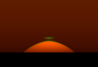 This all works well for inferior-mirage flashes, where the green flash itself
is the only part of the Sun's disk that's visible. But when any part of
the disk but the limb is visible, it's so much brighter than the flash
that the latter is not very conspicuous, as you see here in the
mock-mirage flash at the
left. There just isn't enough dynamic range in a computer display to show
the extremes of brightness in a real sunset, where there's so much more
red light than green.
This all works well for inferior-mirage flashes, where the green flash itself
is the only part of the Sun's disk that's visible. But when any part of
the disk but the limb is visible, it's so much brighter than the flash
that the latter is not very conspicuous, as you see here in the
mock-mirage flash at the
left. There just isn't enough dynamic range in a computer display to show
the extremes of brightness in a real sunset, where there's so much more
red light than green.
You can try to make the reds dimmer by making the haze layer shallow,
which makes things near the horizon darker. But that doesn't help enough.
In this example, seen from a height of 38 m,
the haze scale height was set to 40 m; but —
although this dims the part of the Sun near the horizon quite considerably
— it still leaves the top of the Sun much brighter than the
mock-mirage flash. This approach doesn't work because the flash isn't far
enough above the red disk. If you make the reddening haze dense enough to dim
the top of the disk, it dims the flash even more; and the diffuse light at
the horizon starts to drown it out, too.
So it's necessary to compress the dynamic range somehow. A natural approach
is to do something like what color film does: let the reds
saturate when they're too bright. Although this distorts the colors,
making the red-orange setting Sun turn orange or even yellow, it
at least produces a result that's distorted in the same way color
photographs are distorted.
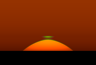 The image at the right shows what you get when you do that. The
brightnesses have been increased by about a factor of 2.7, and the reds
that should have have data values around 690 have been held to 255.
This turns the top of the disk orange (just as a slightly over-exposed
photograph does), and of course flattens the limb-darkening. But at least
the green flash now has a more natural appearance.
The image at the right shows what you get when you do that. The
brightnesses have been increased by about a factor of 2.7, and the reds
that should have have data values around 690 have been held to 255.
This turns the top of the disk orange (just as a slightly over-exposed
photograph does), and of course flattens the limb-darkening. But at least
the green flash now has a more natural appearance.
Incidentally, these examples show why mock-mirage flashes are so seldom
noticed by visual observers: without some magnification, the flash is lost
in the glare of the Sun's disk. (The images shown here have a resolution
of 7.5 seconds of arc per pixel — about 8 times the resolution of the
unaided eye — so they show details visible to an observer using
8× binoculars.)
© 2005 – 2007, 2012, 2021, 2023, 2025 Andrew T. Young
Back to the
GF animation introduction
Back to the
GF home page