To draw the Sun's outline at some moment in a sunset, we need to know how to map the actual or “true” zenith distance of each point on its limb to the place in the sky where it appears — i.e., its apparent zenith distance. The mapping between true and apparent zenith distances is the transfer function.
It's convenient to plot the transfer function with apparent Z.D. on the horizontal axis, and true Z.D. on the vertical one. Actually, because we are only interested in the part of the sky close to the horizon, it's even more convenient to use altitudes instead of zenith distances.
Of course, what we actually calculate is refraction as a function of zenith distance. So a little numerical manipulation is needed to convert a refraction table to a transfer curve. First,
lets us convert the refraction table from zenith distances (Z.D.) to altitudes. Then, because refraction raises objects, their apparent altitudes are greater than the true ones:
But the argument of the calculated refraction table is apparent altitude. So to get the true one, which we need for the transfer curve:
That makes a maximum in refraction become (approximately) a minimum in the transfer curve.
Remember that the refraction — and hence the transfer curve — depends on the height of the eye. So we must specify both a model atmosphere and the height of the observer to get a transfer curve.
It also depends on the refractivity of air, and so on the wavelength of the light used. In these examples, I've colored the curves to indicate the wavelength.
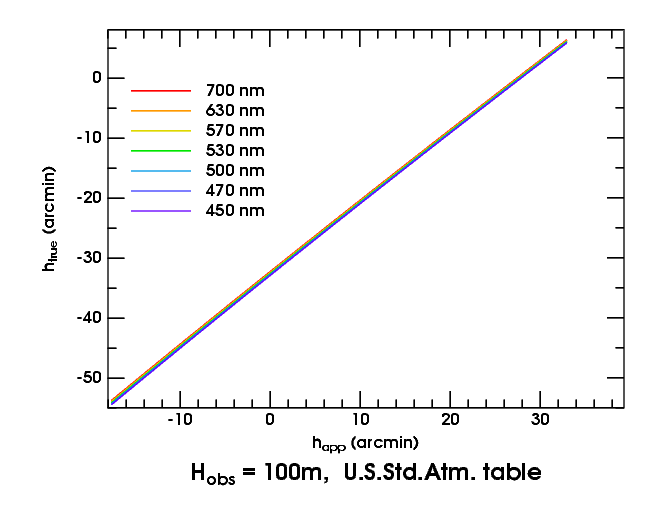
Here are transfer curves at seven different wavelengths for the Standard Atmosphere, as seen from a height of 100 meters above sea level. The left end of the curves is at the apparent horizon.
First, notice that the transfer curves are nearly straight lines. There's no spectacular change in refraction below the astronomical horizon (i.e., to the left of the zero on the abscissa). And the straightness of the transfer curves means the Sun's image is only compressed, not miraged.
Second, notice how small the dispersion (the separation of the curves for different colors) is. You can hardly notice the separation of red from blue at this scale.
It's the separation of the curves that produces the red and green rims. Think of the true Sun as a horizontal band across the graph: the top of the band is the top of the Sun, and the bottom of the band is the lower limb. The top meets the red transfer curve a little to the left of (i.e, at a smaller apparent altitude than) where it meets the green curve. That means the green image is a little higher in the sky; just above the top of the red image, there's a narrow green rim. Similarly, at the bottom, there's a narrow red rim below the bottom of the green image.
Third, notice that there is a slight increase in dispersion
toward the apparent horizon: the red and blue curves are a little farther
apart at the apparent horizon than a degree above it. But that's mostly a
consequence of the greater refraction at the horizon. In short, there's
nothing very interesting about this kind of sunset.
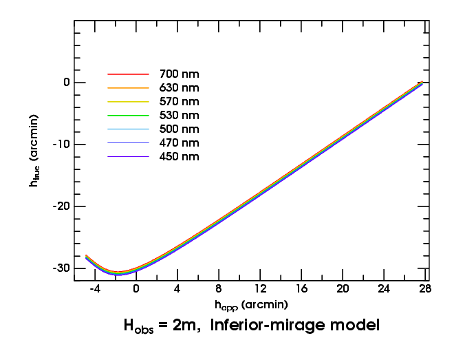
Now consider the inferior-mirage sunset. Here (to the right) are the transfer curves:
Above the astronomical horizon, they look much like the Standard Atmosphere curves. But below it, there's a reversal in slope. That reversal means an image inversion: the inferior mirage, in this case.
The regions of normal (erect image) and reversed slope (inverted image) join smoothly at a minimum. This marks the “fold line”, where the image is infinitely magnified. (In fact, the image magnification at any point is the reciprocal of the slope of the transfer curve there.)
When the lower limb of the Sun is a little below the minimum in the
transfer curves, the slope of the lower left side of the solar
image mimics the shape of the transfer curve, rotated 90°.
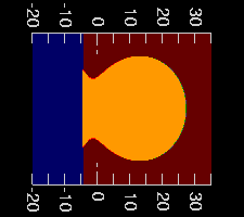 (Here on the left is the image, turned through 90° for comparison.)
That makes the left “foot” of the
Omega shape:
the hook in the transfer curve becomes the corner where the foot
(the inverted image) joins the erect image of the Sun.
If you look closely at the solar image, you can even see that the red
image in this corner is a little higher than the others, just as the red
transfer curve is higher in the transfer plot: the solar limb shows a
narrow red edge at the astronomical horizon (the “0” tick
on the scales in the rotated image).
(Here on the left is the image, turned through 90° for comparison.)
That makes the left “foot” of the
Omega shape:
the hook in the transfer curve becomes the corner where the foot
(the inverted image) joins the erect image of the Sun.
If you look closely at the solar image, you can even see that the red
image in this corner is a little higher than the others, just as the red
transfer curve is higher in the transfer plot: the solar limb shows a
narrow red edge at the astronomical horizon (the “0” tick
on the scales in the rotated image).
And when the top of the Sun sinks to the minimum, there's a moment when the upper limb (at about −31′ true altitude) is just below the minimum in the red transfer curve, but still above the green one. That means the red image of the Sun has vanished, while the green image is at the point of great vertical magnification where the erect and inverted images join: we have the inferior-mirage green flash!
In fact, you can see that the width of the green flash in altitude is just the difference in apparent altitude of the two points where a horizontal line tangent to the red transfer curve cuts the green transfer curve: when the top of the Sun is at the minimum of the red curve, the red light has disappeared from the mock mirage; so green is left. (Strictly speaking, I should have said “yellow” instead of “red”; but the yellow curve is hard to see here.)
This is an example of a general principle:
if there's a smooth
minimum in the transfer curves, there will be a green flash when the Sun's
upper limb reaches that true altitude.
Likewise, when the lower limb reaches a
maximum in the transfer curves, we get a
nice red flash. (The only maximum here
is at the apparent horizon, so the only red flash here occurs when the red lower rim
appears at the horizon as the inverted image begins to rise. This is
visible telescopically, but not with the naked eye.)
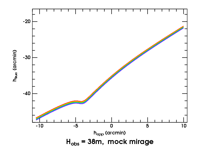
Now let's consider the mock mirage. Here is the transfer plot for the model used to generate some simulations: a weak inversion between 30 and 50 meters, seen from 38 m.
The shallow but obvious minimum is what makes the mock-mirage green flash. This minimum corresponds to a line of sight just tangent to the bottom of the inversion layer. As shown elsewhere, the size of the mock-mirage green flash depends on details of the temperature profile at the bottom of the inversion.
To the left of the minimum in the transfer curve, you see a broad maximum,
which produces the
red flash
that precedes the MM flash.
But this model has such a weak thermal inversion — only 0.8°
— that the mock-mirage red flash is rather small. It's much better
shown with a stronger inversion. To kill two birds with one stone,
let's proceed to a 2° inversion that makes a
duct,
and combine the mock-mirage red flash with the phenomena of ducting.
The first ducted example is relatively mild: only a 2° inversion between 50 and 60 m. But that's enough to supply a rich display of distorted sunsets.
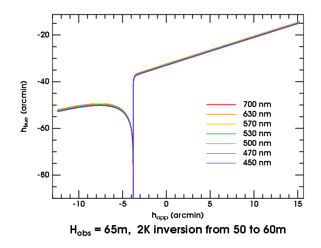
In general, atmospheric structures near eye level produce larger effects than those well above or below it. So let's consider the transfer curves for our weak duct as seen from 65 m height, just 5 m above the top of the duct.
Above the astronomical horizon (i.e., for positive apparent altitudes), this is just like the Standard Atmosphere — a straight line. But below it, the plot falls off a cliff when our line of sight reaches the top of the duct (at about −3.5′). The transfer curves all run off to −∞, because the refraction becomes infinite there.
What has happened? The line of sight from the observer to the sky sweeps down continuously, until it reaches the critical level where ray curvature equals Earth's curvature. As it approaches this critical level, the ray follows the curve of the Earth more and more closely, and the refraction increases without limit; the transfer curve shoots off to negative infinity.
When the ray crosses the critical-refraction level, it discontinuously dips down into and through the inversion layer, passing well below it on the near side of the perigee point, and then tracing a similar path back up through the inversion again, finally emerging far away at a large zenith distance. (Indeed, just below the top of the duct, the refraction is again arbitrarily large.) As we look still lower in the sky, our line of sight passes more obliquely through the super-refractive inversion. Its path length in the inversion decreases, and so does the refraction; the transfer curve rises again, and we see astronomical objects that are really higher in the sky, as we look lower . In short, this is the mock-mirage mechanism at work again; the image is inverted. (See the ray diagram for this ducted mock-mirage model.)
The discontinuity in the ray fan effectively removes a section of the transfer curve around the minimum that produced the ordinary, un-ducted mock mirage. So the transfer curves don't approach one another smoothly on the two sides of the vertical asymptote; there's a jump between the descending and ascending branches of the curves.
Now, the width of the ordinary MM green flash was the width of the minimum in the transfer curve; but the duct has now drawn this minimum out into a fine point, of zero width. So there normally isn't any green flash associated with a ducted mock mirage — although, under extremely clear conditions, a faint green display is possible.
On the other hand, the maximum in the curve is now fat and broad. And it's this maximum that provides the ducted-MM red flash. (See the animation of it here.) The reversed slope of the transfer curves between apparent altitudes of about −4′ and −7′ is, of course, the mock mirage due to the large change in lapse rate at the bottom of the inversion layer.
A few realistic images of this sunset are also available. The second image in that series, at a depression of 34′, shows a wide red rim on the mock mirage below the duct — the remains of the red flash, after it has begun to turn into a more normal image of the lower limb.
The chief feature introduced by the duct is the vertical discontinuity, produced by the layer with critical lapse rate at the top of the duct. These vertical discontinuities are typical of transfer curves produced by ducting. As the top of the duct occurs at almost exactly the same height for all colors of light, the transfer curves all become vertical at nearly the same place in this case. However, the thickness of the duct depends on the refractivity of air, and so is slightly different for different wavelengths.
This variation in duct thickness with wavelength produces several interesting effects. One of them is marginally visible here: the greater separation of the different transfer curves below the duct than above it.
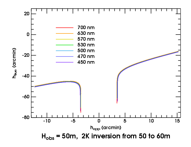
Now let's descend to 50 meters, at the bottom of the inversion, where the ducting effect is strongest. This produces Wegener's “blank strip”, which is shown in realistic simulations here. The two vertical sections of the transfer curves mark the edges of the blank strip; between them, the Sun is not visible.
If you imagine the top of the Sun at a true altitude of −50′ or lower, its entire disk falls on the nearly-vertical edges of the blank strip. That produces a very thin image of the whole Sun at each edge of the strip, as shown in the simulations.
At this height, some wavelength-dependence of the blank-strip width is becoming apparent: it's narrower in red light. But this effect is really prominent when we get near the bottom of the duct.
At the bottom of the duct, the blank strip closes up again. Just above it, the width of the strip is proportional to the square root of your height above the bottom (as can be seen from the square-root scale of dip on the dip diagram). But the square-root function has a vertical tangent at the origin: so small changes in height make very big changes in the width of the strip, just above the bottom of the duct.
This is a different kind of infinite magnification from the one in mirages; but it is just as effective in enhancing refractive effects. It combines with dispersion to magnify the separation of transfer curves for different wavelengths. For the depth of a duct depends on the difference in refractivity across its parent thermal inversion; but that difference is wavelength-dependent.
But the top of the duct is pinned to the top of the inversion, at all wavelengths. Consequently, the height at the bottom of the duct varies markedly with wavelength: it's lower at shorter wavelengths, whose greater refractivity makes the duct deeper.
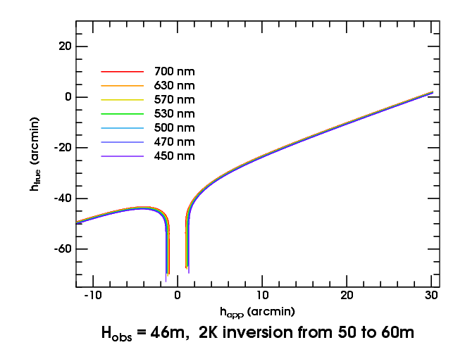
Now look at the transfer curves for our duct as seen from 46 meters, just
above the bottom of the duct. The observer is closer to the bottom of the
duct in red light than in blue, so the blank strip is narrowest for red
and widest for blue light. That gives the edges of the blank strip a red
color, as you can see
here.
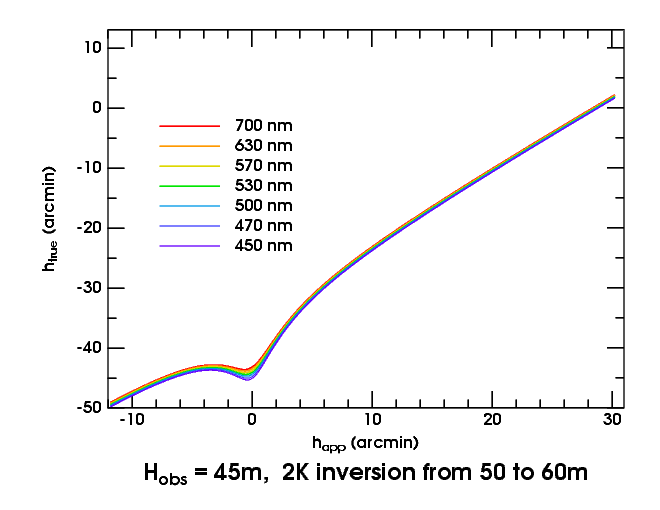
As the observer sinks through the bottom of the duct, the blank strip closes up first at the longest wavelengths, forming a minimum in the transfer curves — which we recognize as creating a green flash. As we descend still further, the minimum becomes shallower and broader, and eventually disappears. But, just below the bottom of the duct, there's a much deeper minimum in green light than in red — as shown in this transfer plot for 45 m height. Because the vertical scale is true altitude, which is nearly a linear function of time near the horizon, that makes the sub-duct flash much longer-lasting than the ones (like the inferior-mirage and mock-mirage flashes) that are just magnified images of the green rim. And, a few decimeters lower, as the minima flatten out, the sub-duct flashes extend over a much greater interval of apparent altitude; so they're big, as well as long-lasting. These are the most spectacular of all green flashes.
Copyright © 2005 – 2009, 2013, 2023 Andrew T. Young
or the
GF pictures page
or the GF home page