Polytropes in Detail
Emden's work
As noted on the
introductory polytropes page,
Robert Emden introduced the word “polytrope” —
first
(1907) in the context of stellar structure, and
later
(1916) in atmospheric physics.
In 1923, he finally applied his model to astronomical refraction in two papers.
The one in
Meteorologische
Zeitschrift
seems to be a shortened version of the full paper, which appeared in
Astronomische
Nachrichten.
I'll summarize that work here, using a slightly simpler notation than
Emden's. It's similar to the treatment on the
previous page, but includes the
proportionality constants, so as to provide actual numbers.
The polytropic index
Instead of developing the theory in terms of the ratio of specific heats,
which is the natural parameter to use in problems of convection, Emden
used the polytropic index n, which let him avoid the restriction to
adiabatic convection, and made the theory more general.
A nice feature of his 1923 papers is to simplify all the relations by
expressing the actual values of state functions in terms of a
characteristic length: the height of the
homogeneous atmosphere,
$$ \mathbf { H_{\scriptstyle 0} = \frac{R\, T_{\scriptstyle 0}}{m \,g} } $$
where: R is the universal gas constant; T₀ is the temperature
at the base of the atmosphere; m is the mean molecular weight;
and g is the (assumed constant) acceleration of gravity.
[If you've forgotten how this relation is derived, see the details on the
hydrostatic equilibrium page.]
On pp. 354–355 of the Met. Z. paper, Emden shows that the
total height H of the whole polytropic atmosphere of index n
is just (n + 1) times this. Notice that if n is
zero, (n + 1) is exactly 1. That's the case for the
homogeneous atmosphere.
So, in general, the height of a simple polytropic atmosphere is
$$ \mathbf { H = ( n + 1 ) \cdot \frac{R\, T_{\scriptstyle 0}}{m \,g} } $$
At this height, the pressure, temperature, and density of the model all
become zero. (This is physically impossible, but is a property of such
simple mathematical models.)
Emden also shows that the vertical temperature gradient dT/dh is
constant. Its magnitude is T₀ divided by the whole height
(n + 1)(R T₀)/(m g), and its sign is negative.
That's \(\mathbf{-m\,g/[(n+1)\!\cdot\!{R}] }\) .
(The temperature cancels out here, as it must, because the gradient is
constant, while the temperature varies with height.) The conventional
lapse rate
Γ is just the negative of this:
$$\mathbf {\Gamma = -\, \frac{d T}{d h} = \frac{m \,g}{ (n + 1 ) R } } $$
which of course is independent of height or temperature, if g is
constant.
The isothermal atmosphere has \( \mathbf {\Gamma = 0} \), which is
possible only if n is infinitely large. Emden showed that the
polytropic expressions for large integer values of n are a
well-known series that converges to the exponential function, so that the
density and pressure decay exponentially with height in this case
(neglecting the slight change in g with height). If the variation
of g with height is considered, Emden showed in his 1923
Met. Z. paper that a fixed polytropic index
corresponds to a constant ratio of lapse rate to g. In modern
terms, that means a constant geopotential lapse rate.
In both of the 1923 papers, Emden included a convenient table of
astronomical refractions for eight values of n from 1 to infinity.
The A. N. paper also has a table of model heights and
lapse rates for the same eight polytropic indices. (This is abbreviated
from a longer table with 14 values of n in the 1916
Met. Z. paper.) He found that the average atmospheric
structure was nearly a polytrope of index 5, for which the total height
would be six times the homogeneous height, or about 48 km. (The
“Standard Atmospheres”
used today all have a tropospheric lapse rate of 6.5°/km,
corresponding to a polytropic height of 44.330769230769 km. [The
ridiculous number of digits is due to the particular values adopted for
the physical constants used.]) The constants adopted by the United States
Standard Atmospheres of 1962 and 1976 correspond to
n = 4.25587611327849; the more recent (1993) ICAO model
has n = 4.25587974247581744045... because it uses a
slightly different value for the gas constant of dry air. These values
for n differ by less than 1 part per million.
The range of observed lapse rates in the real atmosphere far exceeds the
range in Emden's table; in particular, on clear nights at temperate
latitudes there is normally at least one thermal inversion in the lowest
few hundred meters. Emden was aware of nocturnal inversions, but did not
treat them in detail. However, he did point out that a thermal inversion
corresponds to a value of n more negative than − 1.
Polytropic profiles
On p. 355 of his
1916 paper,
Emden summarizes the basic relations among the state variables as
functions of height h, in terms of the polytropic index n
and the full height H of the single-polytrope model. For the
temperature, he gives:
$$ \mathbf {T = T_{\scriptstyle 0} \left( 1 - \frac{h}{H} \right) } $$
for the density:
$$ \mathbf {\rho = \rho_{\scriptstyle 0} \left( 1 - \frac{h}{H} \right) ^n } $$
and the pressure:
$$ \mathbf {p = p_{\scriptstyle 0} \left( 1 - \frac{h}{H} \right) ^{(n+1)} } $$
and the subscript 0 implies the level where \(\mathbf {h = 0} \).
These power-law profiles are the basis for practical calculations in
polytropic layers when a real temperature profile is approximated by a
series of linear segments, so that each layer has its own polytropic index.
The height in every layer is measured from the base of the layer.
Such atmospheric models are often called piecewise
polytropic.
Finding n from observations
Notice that the temperature profile (or, equivalently, the lapse rate) by
itself does not explicitly involve the polytropic index. All the physics
of gravity and gas constant is hidden in the height H, which also
conceals the polytropic index. However, if we have both temperature and
pressure measurements at two different heights, we can in principle
determine both the height H and the index n.
Because the equation of state is a simple power law, the basic polytropic
condition that p is a power of ρ also makes each of them a
power of T. For example, it's obvious from the equations above
that p is just proportional to \( \mathbf { T^{ (n+1) } } \). If
we were to plot p as a function of T on log-log graph paper
(as was done in the days before computers), we would get a straight line
with a slope of \( \mathbf { (n+1) } \) .
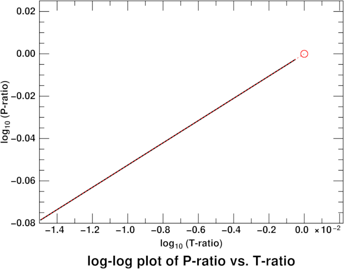 Here's such a graph for just the lowest 1500 meters of the U.S. Standard
Atmosphere. The black line uses the tabulated values at every 50 meters
of height, and the red dashed line is calculated from just the 1500-meter
point and the value at the surface, which is circled. The two lines
coincide perfectly.
Here's such a graph for just the lowest 1500 meters of the U.S. Standard
Atmosphere. The black line uses the tabulated values at every 50 meters
of height, and the red dashed line is calculated from just the 1500-meter
point and the value at the surface, which is circled. The two lines
coincide perfectly.
So, if we have T and p values for two heights, we can get
that slope very simply. Let the data for the two heights be labelled with
subscripts 1 and 2. Then the slope of the line is just
$$ {\mathbf { n+1 = { \left(
\frac{ \log p_{\scriptstyle 1} - \log p_{\scriptstyle 2} }
{ \log T_{\scriptstyle 1} - \log T_{\scriptstyle 2} }
\right) } } } $$
— but of course, \(\mathbf {( \log a - \log b)}\) is just
\( \mathbf {\log (a/b)}\). So we can replace two expensive
logarithm evaluations with cheaper divisions:
$$ {\mathbf { n+1 = { \left(
\frac{ \log ({{p_{\scriptstyle 1}}/{p_{\scriptstyle 2}}) } }
{ \log ({{T_{\scriptstyle 1}}/{T_{\scriptstyle 2}}) } }
\right) } } } $$
and we can obviously get n itself by subtracting 1 from that
expression. And, as the height of the whole polytrope is just
\( \mathbf { (n+1) } \) times the height of the homogeneous atmosphere,
once we have that, we have H.
In making the plot, I used the ratios of temperatures and pressures at the
upper point to their values at the lower one. But it's immaterial whether
point 1 lies above or below point 2. And it also makes no difference
whether we choose natural or common (base-10) logarithms, as long as we
use the same kind of logs for both numerator and denominator.
Application: barometric hypsometry
Supposing that we have found n and H from pressures and
temperatures, we can use them to find the height difference between points
1 and 2. (Emden does this on p. 356 of his 1916 paper.) Densities
are hard to measure, so radiosondes used to provide only temperature and
pressure data, with pressures measured directly by an aneroid barometer.
(Indirect methods using GPS heights have been used since 2014, but the old
method is still used to re-analyze older data.) So it's usual to solve
the pressure equation for the height difference h.
If we assume that \( \mathbf { {{p_{\scriptstyle 0} } } } \) is the
pressure at the lowest point in a layer (not necessarily the surface), the
height difference across a polytropic layer of index n is
$$ \mathbf {h = H \left[ { 1 - { \left( p/p_{\scriptstyle 0}
\right)^{{\scriptstyle \frac{1}{n + 1}} \; } \;\, } } \right]} ,$$
and we can just add up the heights of successive layers, from the ground up.
If a layer is thin, the ratio of the pressures is close to unity, so its
logarithm is close to zero. The same is true for the temperatures; so
n isn't very accurately determined. Then the polytropic height
H is also uncertain. Partly for this reason, the exact polytropic
determination of heights never became standard practice in meteorology or
aviation. Unfortunately, the practical need to do something
to get roughly realistic heights allowed an empirical procedure to become
entrenched, long before better physical (i.e., polytropic) models were
available.
So the traditional approach to finding heights from pressures uses a
systematically incorrect method that goes back two centuries to Laplace's
Mécanique Céleste (1805) — where the temperature was
assumed constant. Various artificial and unrealistic modifications of the
constants involved, such as the acceleration of gravity and the gas
constant, have become fixed in this process, which is described in
meteorology textbooks as “the” hypsometric equation.
Laplace's hypsometric equation had been used for more than a century to
estimate the heights of mountains, despite its weaknesses, before
polytropes were invented. After just a few years of use, it became
evident that the calculated heights had both diurnal and seasonal
systematic errors that varied from place to place. Today, it's obvious
that these effects were the natural result of changes in the lapse rate
from day to night and from summer to winter; but in the 19th Century this
was not understood.
The physically incorrect assumption of an isothermal atmosphere forced the
adoption of a fictitious “mean temperature”. But the mean adopted has
always been the simple arithmetic mean, which is physically wrong for any
realistic model — as was pointed out by
Diehl
in 1925. (He favored the harmonic mean.) However, Laplace's isothermal
rule was by then too firmly established to be replaced.
The use of adjusted constants to get answers closer to
real-world measurements is similar to the procedure used by Simpson
(1743),
Bradley [as published by Maskelyne in
1763 and
1764],
and
Tobias Mayer
[again, as published posthumously by Maskelyne in 1770,
and then explained in more detail by him in
1787],
to obtain better refraction tables near the horizon
from the assumed linear decrease in density with height.
Such artifices were needed before the gas laws were fully understood.
Application: prescribed temperature profile
It should be obvious now that the heights reported in radiosonde profiles
are not very accurate. But if we want to specify some artificial model
atmosphere, we can just make up heights and temperatures to see the
effects of various assumptions. And one such fictitious model is the
misleadingly named
Standard Atmosphere,
whose assumed tropospheric lapse rate of exactly
6.5 Celsius degrees per kilometer was proposed in
1919.
With the lapse rate specified, it's trivial to find the polytropic index,
because the lapse rate is just the temperature at the base divided by the
total height H of the polytrope; and the height of the polytrope is
exactly \( \mathbf { (n+1) } \) times the height of the homogeneous model.
So from
$$ \mathbf { \Gamma = \frac{ T_{\scriptstyle 0}}{H} } $$
and
$$ \mathbf { H = ( n + 1 ) \cdot \frac{R\, T_{\scriptstyle 0}}{m \,g} } $$
we have
$$ \mathbf { ( n + 1 ) = \frac{m \,g }{R\, \Gamma} \; }. $$
This is the relation between the lapse rate \( \Gamma \! \) and the
polytropic index, n. It does not depend on height, or on
conditions at the base of the polytrope. The only other parameters used
here are the mean molecular weight and the acceleration of gravity.
However, adopting a different value for the gas constant or the molecular
weight changes the numerical value of n.
Notice that an isothermal layer has zero lapse rate, and an infinite
polytropic index. The large range in actual lapse rates near the ground
produces a large range in n, and the systematic variations in
conventional barometric hypsometry.
Copyright © 2025, 2026 Andrew T. Young
Back to the ...
introduction to polytropes page
or the
temperature profiles page
or the
refraction calculation page
or the
GF home page
or the
website overview page