Ducts and Anomalous Horizons: False, Double, etc.

Introduction

Back when celestial navigation was the main way to determine a ship's position, mariners measured the apparent altitudes of the Sun and stars above the visible sea horizon, and corrected these apparent altitudes for dip. They were disconcerted when that horizon appeared double, or otherwise appeared peculiar because of unusual refraction effects. The “Mariner's Log” section of Marine Observer contains many references to such phenomena.

If the sea horizon appeared double, which of the two was the right one to use? Their separation might be several minutes of arc, corresponding to an error of several miles in a ship's position — a serious error in navigation. And, if the horizon was behaving strangely, would the usual correction for its dip be correct? These were practical problems for navigators.

Such problems often occur when the observer is in, or near, a duct. And the effects of ducts on the apparent horizon have to be understood in making mirage simulations. So I've had to figure out the details of these effects.

Atmospheric Models with Ducts

Duct structure

Any thermal inversion with a steep enough negative lapse rate can produce a duct. But the inversion's stability against convection allows considerable variations in lapse rate, even within a few meters of height. When the wind is light, it's common to find an unstable surface layer, capped by a steep inversion. Even without a convective surface layer, the lapse rate may be neutral, or at least not super-refracting, beneath the steep part of the inversion.

In this case, the duct will have two parts. The upper part is super-refracting (i.e., the curvature of a horizontal ray there exceeds the Earth's curvature); the lower part refracts normally, whether its lapse rate is positive or weakly negative. There may also be a normal (or even convective) surface layer below the bottom of the duct. Each of these parts affects the appearance of the horizon differently.

Elevation ordering

Remember that a duct is produced by a thermal inversion strong enough to bend a horizontal ray of light with a smaller radius of curvature than the Earth's curvature. That bending, which requires an inversion steeper than about 0.115°C/m, traps nearly-horizontal rays beneath the top of the duct — which I'll also call “the top of the inversion,” although the lapse rate may be more weakly inverted for some distance above it. It's convenient to assume that the top of the inversion and the top of the duct coincide, even though this may not be strictly true.

A ray that's horizontal just below the top of the inversion leaves the base of the inversion at an angle; so it continues to descend for some distance below the bottom of the inversion, before the curve of the Earth bends away from it, making the ray locally horizontal again. So the bottom of the duct is always below the bottom of the inversion. (See the ray diagrams and the discussion of the depth of the duct, on the duct page, if you haven't been there recently. The bottom of the duct is also shown as a dashed line in my simplified presentation of Wegener's model.)

As I explained on the duct page, several atmospheric regions are stacked up when there is a duct. At the top is the free atmosphere above the duct; then comes the top of the super-refracting thermal inversion that produces the duct. (The top of the inversion is also the top of the duct.) Some distance below this is the bottom of the super-refracting region; for convenience, I usually call this just “the base of the inversion”, although the lapse rate often remains mildly inverted below the bottom of the super-refracting region. Lower still, if the duct is elevated, we can have the bottom of the duct. Finally, if the duct itself is entirely above ground level, there is the surface of the Earth.

These pieces are always stacked up in this order. Some of the lower ones may be missing, if the inversion is low enough: if the duct is “surface-based”, the ground intervenes before a ray that is horizontal just below the top of the inversion becomes horizontal again below the inversion. Or, if the inversion itself extends down to the surface, the inversion is surface-based; then every  ray below the top of the inversion meets the surface obliquely. Because the base of the duct is always lower than the base of the inversion, there cannot be an elevated duct if the inversion is surface-based. Hasse (1960; 1964) investigated the optics of surface-based inversions, and found that the top of the inversion produces a false horizon that he called a Kimmfläche or “horizon surface”.

The optical effects produced depend on geometric relationships among the duct, the observer, and the surface of the Earth. Let's begin with the relative positions of the duct and the surface, and then see what happens as the height of the eye changes in each arrangement. The diagrams in the subsection that follows show the relative heights above the ground of the atmospheric layers involved. (To see the correspondence between these atmospheric structures and the images they present to an observer, we will need to use transfer curves and the duct diagram, which are discussed in the section after that.)

Duct Geometry

There are three kinds of duct, depending on how they're placed, relative to the Earth's surface. Here they are, with the atmospheric layers of different optical properties shown as a color-coded cartoon: the layers with normal (positive — or at least not negative enough to be super-refracting) lapse rates are sky-blue; the upper (super-refracting) and lower (normal) parts of the duct are pink and orange; and the ground is nearly black. These colored cartoons represent vertical structure within the boundary layer.

Type 1: Duct completely above the surface.: This is an elevated DUCT.
←normal lapse rate above duct
←inversion: upper part of duct
←normal lapse: lower part of duct
←normal lapse rate beneath duct
Type 2: Inversion completely above the surface; duct touching the surface.: This is an elevated INVERSION, but a surface-based DUCT.
←normal lapse rate
←inversion: upper part of duct
←normal lower part of duct
Type 3: Inversion touching the surface.: This is a surface-based INVERSION.
←normal lapse rate
←inversion

Note: this is the only case treated by Hasse (1960).

The terms involving combinations of “elevated” or “surface-based” with “inversion” or “duct” are easily confused. So let's just keep track of the types by number, from 1 to 3 (from highest to lowest inversion).

Understanding the Duct

To understand the ray paths in a model containing a duct, the dip diagram can be very useful. It may be helpful to review the features of a ducted model, showing how the features of its dip diagram arise, before dealing with the ray-tracing phenomena. So here's a brief review of my smoothed-inversion model with an elevated duct — a Type-1 model. Let's begin with the temperature profile.

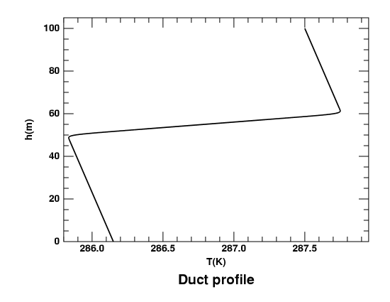
Temperature profile:

In the ducted model I've used most for sunsets and mirages, the 2° thermal inversion that produces the duct extends from 50 to 60 meters height. That makes its lapse rate −0.2°C/m, almost twice the threshold value required to produce a duct.

The diagram at the left shows the temperature profile in the lowest 100 m of this model. As is usual in meteorology, height is plotted on the vertical axis.

Elevated-duct layer boundaries

←T
←B
←D

For comparison, here is the cartoon showing the layers of the Type-1 (elevated-duct) model again, but with the layer boundaries marked, instead of the layers themselves. The top of the inversion is at T, corresponding to the right-hand corner in the temperature profile; the bottom of the inversion is B, corresponding to the left corner; and the bottom of the duct is D, which is near 45 meters — but no feature exists in the temperature profile at that height.

Density profile:

T B ←D

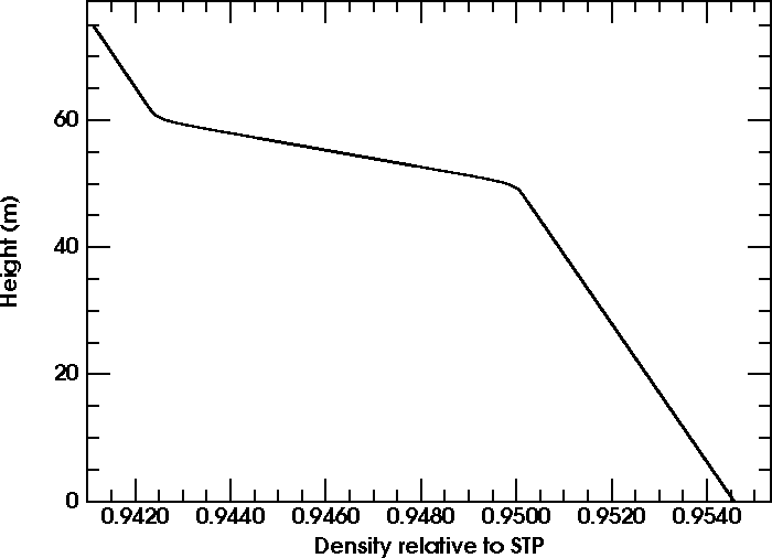
To trace rays through a model atmosphere, we must convert its temperature profile to a refractivity  profile. An intermediate step is to generate the density profile; the refractivity is (to a very good approximation) proportional to the density of the gas.

The density can be calculated from the temperature by assuming hydrostatic equilibrium — i.e., the pressure at each level is just the weight per unit area of the overlying column of gas. (The well-known RGO program shows how this can be done for both isothermal and polytropic layers.)

The adjacent graph shows the resulting density plot for the duct model. As before, height is on the vertical axis, and the actual dependent variable is on the horizontal axis. The letters T, B, and D denote the Top of the inversion, the Base of the inversion, and the bottom of the Duct, respectively. As before, there is no feature in the profile that corresponds to the bottom of the duct.

The rapid decrease in density with height shows that this atmosphere is stably stratified. Notice the stronger stratification in the inversion, between B and T.

Now that we have the density profile, we can turn it into a refractivity profile, as the refractivity (n − 1) is very nearly proportional to the density. Adding 1 to the refractivity gives n, the refractive index. And multiplying n by R, the distance from the center of curvature, gives the product nR, which is the ordinate of the dip diagram.

Dip diagram:

B D T

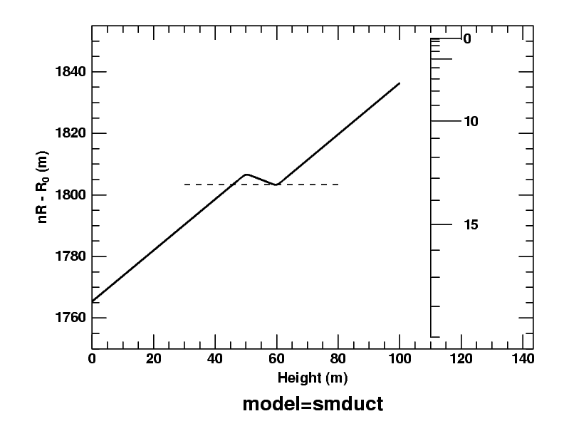
Here's the dip diagram for the same model: a plot of the refractive invariants of horizontal rays as a function of their heights. Notice that the height scale here is on the horizontal axis. Don't let this change of orientation confuse you.

As before, the top and base of the inversion are marked by T and B, and the bottom of the duct is at D. In the dip diagram, the point D on the model-atmosphere curve is at the same ordinate as the top of the duct, as shown by the dashed horizontal line in the figure. The duct covers the whole range of heights from D to T.

The dip scale, in minutes of arc, which is inserted just at the right of the model curve, is explained on the dip diagram page. It can be used to show that the dip of the duct edges D and T (where the dashed line meets the solid curve) — as seen from B, the base of the inversion — is 3 or 4 minutes of arc. That's the half-width of Wegener's “blank strip”, which is centered on the astronomical horizon.

Finally, because nR has the same value at the top (T) and bottom (D) of the duct, any ray passing obliquely across the duct has the same inclination to the local horizon at both those heights. (This follows from the refractive invariant.)

I intended to offer ray diagrams and simulated images here, but found that my ray-tracing programs have numerical difficulties when the ray curvature is close to the Earth's curvature. So this page offers just a hint of the complications that ducts can produce. I hope it's helpful, even though woefully incomplete.

Back to the ...
dip-diagram page

or the distance to the horizon page

or the general ducting page

or the astronomical refraction page

or the GF home page

or the Overview page